
CRISPR Edit Inference
Work out what a CRISPR edit actually produced, from a pair of Sanger reads.
| Reached by | Tools → CRISPR Edit Inference (ICE) |
What it does
A CRISPR-edited pool is a mixture. Some chromosomes were never cut, some carry a one-base insertion, some a four-base deletion, some a larger lesion — and a single Sanger read across that mixture is all of them superimposed. Past the cut site the chromatogram stops being one sequence and becomes a sum of shifted sequences, which is why a read that looked clean up to the guide turns into a wall of overlapping peaks after it.
Edit inference takes that wall apart. You give it the edited read and an unedited control read of the same amplicon, plus the guide you used. It builds every plausible edit outcome around the predicted cut — each insertion and deletion up to a size you choose, and an HDR product if you supply the repair template — simulates the chromatogram each outcome would produce, and then finds the mixture of those outcomes that best explains the trace you actually got. What comes back is a spectrum: which alleles are present and at what proportion, how much of the pool is still wild type, and how much of it has a frameshift.
Three numbers summarise it:
- ICE — the percentage of the pool that carries any edit at all (the indel rate).
- KO — the knockout score: the fraction carrying a frameshifting indel (not a multiple of three), which is the number that matters if the point of the edit was to disable a gene. A pool can be 90% edited and a poor knockout if most of those edits are in-frame.
- R² — how well the fitted mixture reproduces the observed trace. This is the trust dial. A high ICE with a low R² is a decomposition to disbelieve, not a result to report.
When you'd use this
Used in: Design a CRISPR guide, check where else it binds, and measure the edit you got
You have transfected or injected, amplified the target locus by PCR, and sent the product for Sanger sequencing along with the same amplicon from unedited cells. The route is:
- Design the guide — CRISPR Guide Design, which also gives you the verification primers to amplify the locus afterwards.
- Edit, amplify, sequence at the bench. Send the control alongside; without it there is nothing to decompose against, and a control from a different amplicon will not do.
- Infer the edit — this tool. One pair for one sample, or a whole plate in one press.
- Take the pool forward, or don't. The spectrum tells you whether to clone out single alleles, pick a different guide, or accept the pool.
It answers the question a gel cannot: a T7E1 or heteroduplex assay tells you that something was cut; this tells you what the edits were and in what proportions, from a read you were going to take anyway.
What this computes
The composition of an edited pool, taken out of a single Sanger read that is all of it superimposed.
- The allele spectrum: which edit outcomes are present and at what proportion — each insertion and deletion up to the size you choose, plus an HDR product when you supply the repair template
- How much of the pool is still wild type, which is the number a screening decision turns on
- The predicted cut position the outcomes were built around, from the guide you supply
- A simulated chromatogram per outcome, and the mixture of them that best explains the trace you actually got — the fit is over the real trace, not over base calls derived from it
- The fit quality, so a spectrum that explains the read poorly is visibly poor rather than reported with the same confidence as a good one
- An uncertainty for every allele: each share is refitted without the Lasso's shrinkage and reported with a 95% confidence interval and a p-value, and the edited share is also given as a fraction of the signal the fit explains, so a poor fit does not read as a low editing rate
- The bases inside an insertion, where the trace determines them, and
nwhere it does not - A warning when signal sits at the edge of the searched sizes, judged as one group by its own test, because an edit larger than the largest size searched spreads into several small shares
- Which alleles the trace cannot tell apart: two outcomes whose expected traces are so alike (a variance inflation factor above 5) that only their sum is measured are reported as one group, with the group's share and its 95% interval, and the split between them is said to be unmeasured
- Each guide's own answer in a multiplexed edit: the share edited at that cut, its indel spectrum there alone, and the alleles edited at it and at another cut, which are listed under both guides rather than folded into either
- Base edits, when you ask for them: every single-base change on the PAM-distal side of each cut is fitted beside the indels, each reported with its protospacer position, the control base it sits on, the change on the guide's strand, its share and interval, and the share of the pool carrying any base edit as a range (a Sanger read cannot say whether two conversions sit on the same molecules)
- Two independent reads of the same pair, beside the fit and never averaged into it: TIDE once per guide, and a breakpoint decomposition (tracy) whose one or two allele sizes are compared with the fit's top sizes, with a disagreement stated as one
- Every coordinate counted from 1 on the control read: the cut is "after base n", and both windows are given as first and last base, inclusive
- From TIDE: an abundance and p-value per indel size, the base composition of the +1 insertion, how much of the aberrant signal past the break fits no indel size in the range (flagged when it exceeds the read's own noise before the break), a second decomposition up to a second divergence further along the read, and a knock-in share when you supply the donor
- A reading of the result, written from the result — what this pool is in one sentence, whatever undermines that conclusion for this pair of traces, and the full derivation: the model, the estimator, the policies that placed the cut and the windows, the two files by name, and what the uncertainty is. It is generated per run, so two pools never share a reading; see How to read the reading
It needs an unedited control read of the same amplicon. Past the cut site an edited read stops being one sequence and becomes a sum of shifted sequences; the control is what the shifted copies are measured against, and without it there is nothing to decompose.
Where it lives
Tools → CRISPR Edit Inference (ICE) in the right rail. The panel takes its two traces from any file in your projects — a control sequenced once and reused across a whole programme does not have to be copied into each project to be used.
Selecting a guide sequence in an open construct and using Use selection fills the guide field from the canvas. When the construct on screen actually contains that guide, the inferred cut site is marked on the map; when it does not — the common case, because the thing on screen is often the trace itself — the panel says so explicitly rather than drawing a cut at a guessed position, and the analysis still runs against the control read's own base calls.
Inputs and outputs
Takes: two Sanger chromatograms (.ab1, .abi, .scf, .ztr) covering the same amplicon in
the same direction — one unedited control, one edited — and one or more guide sequences (RNA is
accepted and transcribed to DNA). Optionally an HDR donor / ssODN, which turns on the knock-in
readout. For a plate: any number of edited traces, and a definition file naming the pairs.
Gives back: the ICE / KO / R² summary, the full indel spectrum from −2× to +1× your chosen maximum indel size (including the zeros, so the shape is visible), each fitted allele with its sequence around the cut and its relative abundance, the HDR percentage when a donor was given, the independent ICE-D discordance estimate, and the per-base discordance profile the fit rests on.
Refuses, with the reason: a guide that is not nucleic acid is caught before the run, next to the field you typed it into. A guide that cannot be located in the control read stops the analysis and says which guide — because a guide absent from the control means the control is the wrong amplicon, the wrong direction, or the wrong sample, and every number downstream of that would be confident and wrong. A trace too poor to align is reported as such rather than fitted anyway.
How to read the reading
Both methods report a Reading under their numbers, and it is three things in order: the conclusion, then whatever undermines it, then the machinery behind it under How this was derived.
It is written from the completed run, never from the controls on screen. Move a knob and the result clears rather than sitting there explained by parameters that no longer produced it — so the reading you are looking at always describes the numbers beside it.
The conclusion says which of three things the pool is. No edit at all; one clean outcome; or a mixture, in which case it names how many alleles carry the signal and which one leads. It states the knockout fraction separately, because edited and knocked out are different questions: a 3 bp deletion is an edit and is in frame.
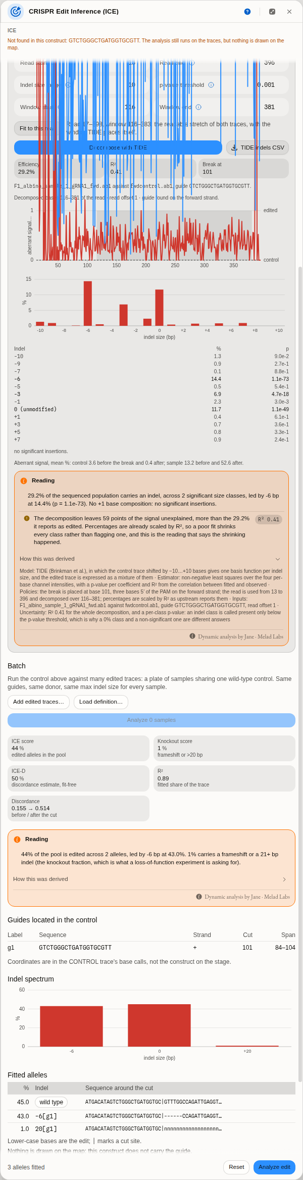
The same two traces, read twice. TIDE reports 29.2% at an R² of 0.41 and the reading says what that costs: the decomposition leaves 59 points of the signal unexplained, more than the edit it reports. Below it, ICE on the same pair — 44% of the pool edited and 1% knocked out, because the −6 bp allele carrying 43% of it is in frame. Neither number is wrong, and neither answers the other's question.
The caveats are earned, not boilerplate. A run with nothing wrong with it carries none, and that is informative. When one appears it is because two numbers from your own run came out the wrong way round — never because a value crossed a threshold, because neither method publishes one. What you may see:
- The fit leaves more of the trace unexplained than the edit it reports. Percentages are scaled by the fit, so the leftover is signal the modelled outcomes do not account for — not extra wild type. This is the caveat that separates a poor decomposition from a poor edit.
- The two estimates disagree by more than the smaller of them. ICE-D is computed from disagreement with the control alone and never sees the fit, so a gap is information: an indel larger than the range you set, or a second unmodelled break.
- An outcome sits at the edge of what was modelled. Then the range you chose decided the answer, not the biology. Raise it and re-run to see whether the peak moves.
- Synthego's own analysis notes, quoted as the library wrote them — a missing PAM, a control trace poor enough that the inference window had to be shortened, multiple donor integration sites.
For TIDE, the caveats are its authors' own quality checklist, applied to your numbers instead of printed as a list for you to apply by eye. The aberrant-signal means it reports are the input to three questions: does the sample diverge from the control after the break more than the control diverges from itself; does the sample's own signal rise downstream of the break at all; and is the control's signal evenly distributed across it. A read that fails one of those is a sequencing problem rather than an edit, and the reading says which.
What no reading will give you is a pass mark. There is no published R² below which an ICE or TIDE result should be discarded — we looked, and the paper of record is paywalled, its preprint unavailable, and the vendor's own guidance pages gone. So the fit is reported, its consequence for your percentages is spelled out, and the judgement stays yours. Treat a figure claiming a cutoff with suspicion unless it cites one.
Worked example
Open CRISPR edit inference (ICE) from the lobby's sample projects. It carries four real
chromatograms from a published cane-toad tyrosinase editing experiment (CC-BY-4.0, Zenodo 15945185),
along with the guide the depositors used, GTCTGGGCTGATGGTGCGTT.
- The panel opens seeded with
fwdcontrol.ab1as the control,Partial_albino_1_gRNA1_fwd.ab1as the edited read, and that guide. Press Analyse edit. - Read the summary. ICE 50, R² 0.93 — half the pool is edited, and the fit is good enough to believe the breakdown.
- Read the spectrum. Twelve alleles: 43% still wild type, then two different four-base deletions at 19% and 12%, a −7, a −17 and a tail of rarer outcomes. Two distinct −4 alleles is a real and common result — the same length lost in two different places is two different chromosomes, and only a decomposition shows it.
- Swap the edited trace for
F1_albino_sample_1_gRNA1_fwd.ab1and run again: ICE 43, R² 0.88, and the spectrum collapses to two things — 45% wild type and 42% of a single −6 deletion. Six bases is a multiple of three, so this is an in-frame lesion: a well-behaved heterozygote whose knockout score is low precisely because its edit does not frameshift. - Now run the negative control.
Partial_albino_2_gRNA1_fwd.ab1came from an animal that looked partially albino. ICE 0, R² 0.99: 99% wild type. The phenotype was not from an edit at this site. This is what a genuinely unedited sample looks like, and it is worth running once so you recognise it.
Batch: a plate in one press
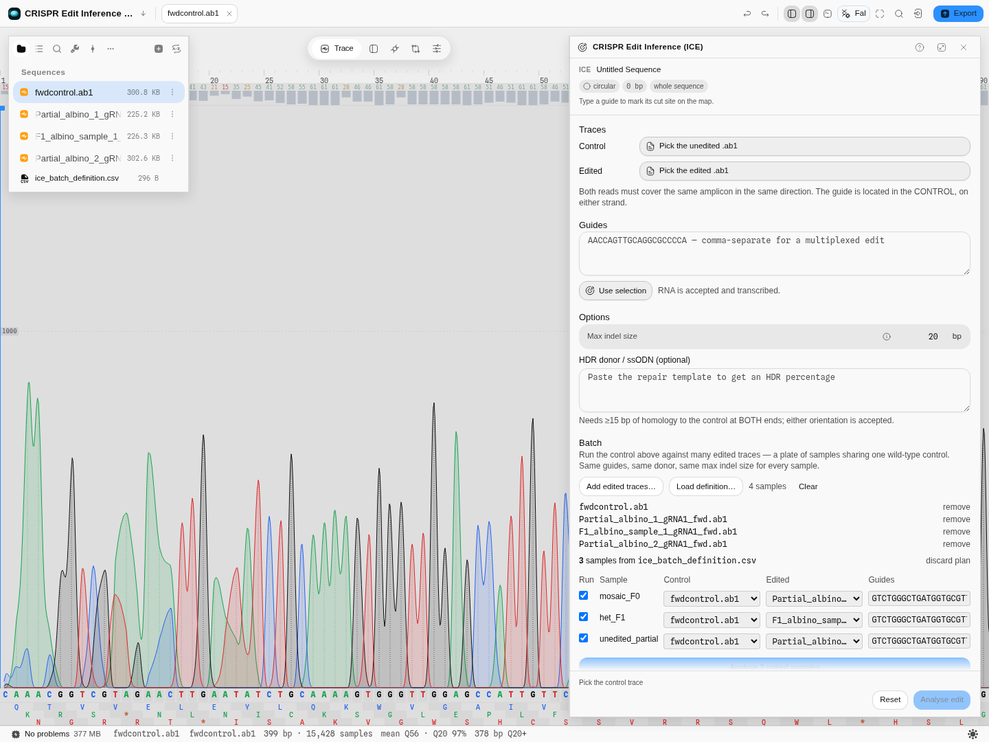
The plan the definition file proposes, before anything runs: each sample names its own control, its own edited read and its own guides, and every one of those is editable here.
A definition file is a small table with one row per sample and these columns:
| Column | Holds | Also accepted as |
|---|---|---|
Label | the sample name every result is reported under | — |
Control File | the unedited read for this sample | Control |
Experiment File | the edited read for this sample | Experiment |
Guide Sequence | one guide, or several comma-separated for a multiplexed edit | — |
Donor | the repair template, when the sample is a knock-in | Donor Sequence |
Save it as .csv, .tsv or a spreadsheet. The steps:
- Load the traces — Add edited traces…, and select every read the plate uses, controls included. Pairing is by filename, so the files themselves have to be present.
- Load the plan — Load definition…. In the sample project,
ice_batch_definition.csvis already there. - Check the pairing. This is the step that matters, and it is why nothing is inferred from filenames: a mis-paired sample does not fail, it returns a confident wrong number. Each row shows the control and edited read it resolved to; change either from the dropdown, edit the guides, or untick a row to leave it out. A filename the sheet names but you have not loaded is listed by name rather than quietly dropped.
- Run it — Analyse N paired samples.
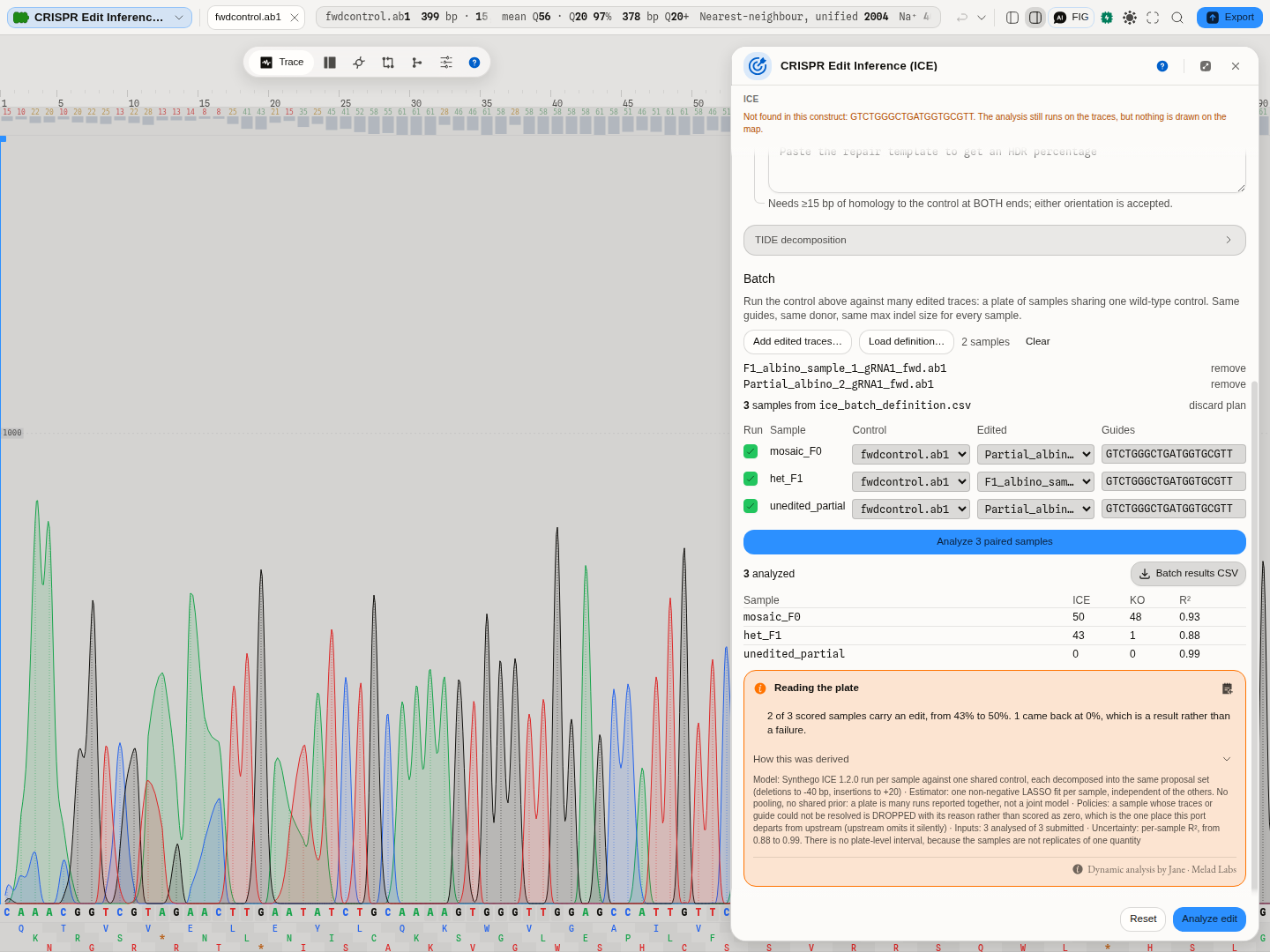
The same three samples, decomposed: ICE 50 / 43 / 0 with R² 0.93 / 0.88 / 0.99 — the values step 2 through 5 of the worked example produce one at a time.
Every row that ran appears in the table with its ICE, KO and R², and every sample that could not run appears underneath it with the reason. A short table is always explained, never just short. The whole result exports as one CSV.
A second opinion: TIDE
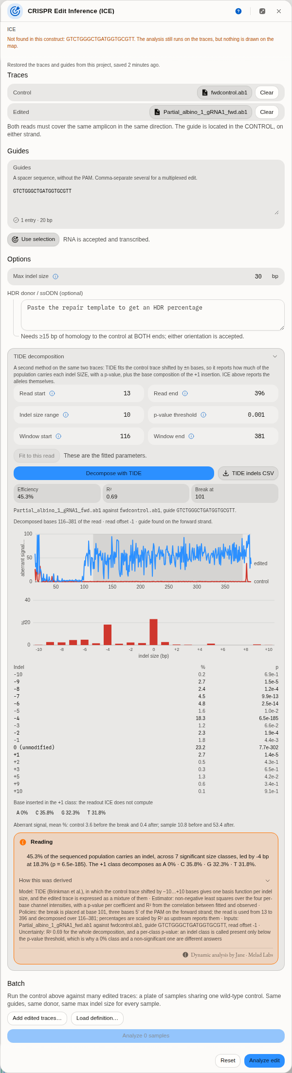
The same two traces as the worked example, decomposed by TIDE instead, on a window fitted to the read: 45.3% edited, R² 0.69, a −4 carrying 18.3%, and the base composition of the +1 insertion. The plot at the top is the one to read first — the control (red) stays flat across the whole read while the edited sample (blue) is flat to the cut at base 101 and jumps to 40–80% after it. That step IS the edit.
Edit inference has more than one published method, and they do not answer quite the same question. Alongside ICE the panel runs TIDE — Tracking of Indels by DEcomposition — on the same two traces and the same guide, so you do not supply the files twice.
What is different, and why it is worth running both:
| ICE | TIDE | |
|---|---|---|
| What it fits | the candidate edited sequences | the control trace, shifted by ±n bases |
| What it reports | alleles, each with its sequence | an abundance per indel size, each with a p-value |
| Only it gives you | multiplex, base editing, the named alleles and their sequences | the base composition of the +1 insertion, and how much signal no size in the range explains |
ICE tells you which alleles are in the pool. TIDE tells you how much of the pool carries a four-base deletion, and how confident that is.
Run both on the three bundled samples and the comparison is worth more than either column:
| Sample | ICE | TIDE | R² (ICE / TIDE) |
|---|---|---|---|
| mosaic F0 | 50 | 45.1% | 0.93 / 0.68 |
| clean heterozygote | 43 | 29.2% | 0.88 / 0.41 |
| genotypically unedited control | 0 | 15.6% | 0.99 / 0.92 |
The TIDE column was run on the hand-set window 20–380. The same F0 pair on the window Fit to this read picks (13–396, decomposing 116–381) gives 45.3% at R² 0.69 — the size of the shift you should expect from moving the window, and a reminder to record the window beside any percentage you quote.
Two lessons are in that table, and both are about how to read a decomposition rather than about which tool is better.
TIDE fits this locus less well (R² 0.68 and 0.41). One class per indel size is a coarser model than one candidate per allele, and this target has two different four-base deletions that TIDE necessarily merges into a single −4.
And on the sample with no edit in it, TIDE reports 15.6% at a perfectly respectable R² of 0.92. This is the single most important thing to understand about any trace decomposition: a good fit is not evidence that an edit happened. Given a trace with nothing to explain, the method will still distribute signal across its classes and report a number. What tells you the truth on that sample is the aberrant-signal readout — the edited read barely separates from the control after the cut — and that is why it sits next to the percentage rather than behind it. Run the negative control once, so you know what "nothing happened" looks like in both methods.
The +1 insertion readout has no equivalent in ICE. Cas9's most common single-base insertion is a duplication of the base 5′ of the cut, so its composition is a fingerprint of the repair rather than a curiosity: a +1 class that is 80% one base is behaving as the literature describes, and one that is evenly split across all four is a sign the +1 signal is noise being fitted.
Running it
-
Open TIDE decomposition below the ICE options. It uses the control, the edited trace and the first guide already in the panel.
-
Set the read window, or press Fit to this read. The defaults are the published tool's own — read start 100, read end 700, decomposition window 115–685, indel range 10, p < 0.001 — and they are deliberately left alone, because they are the settings every published TIDE number was produced with. They assume a read whose cut site is comfortably past base 100. The bundled cane-toad amplicon cuts at base 101, so the defaults cannot decompose it: the alignment stretch runs from the read start to one indel range before the cut, and there is nothing between base 100 and base 91.
The panel says so before you press anything, and offers the way past it. The button is disabled and the reason sits under it, so this is something you read while setting the window rather than something you discover from a failed run. It does not name a read start to try: the obvious one — 91, just before the cut minus the indel range — leaves a single base to align on and refuses a second time. Only a fit computed from your reads can name a start that runs.
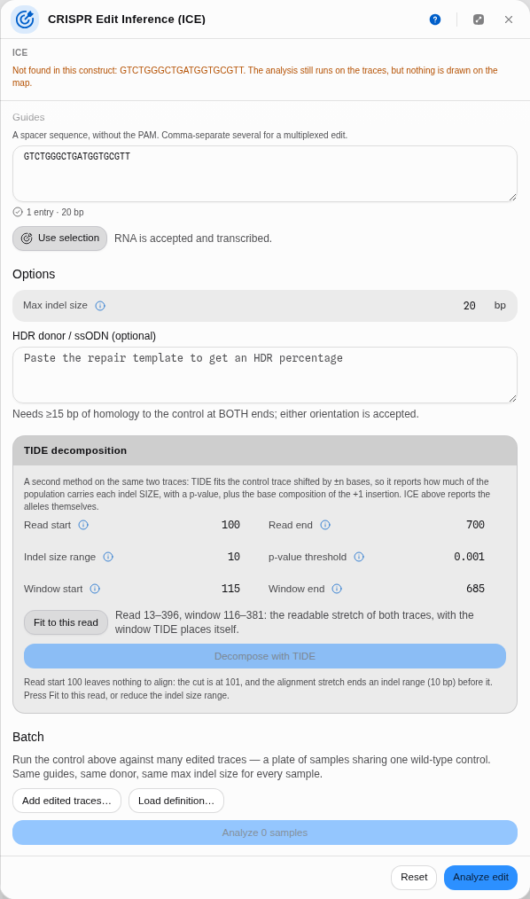 At the default read start the panel refuses in place: it names the cut (101) and the indel range it has to clear (10 bp), and beside it Fit to this read offers the window it would set — read 13–396, decomposing 116–381 — with Decompose disabled until one of the two happens.
Fit to this read does the arithmetic for you, and it is worth knowing what it picks rather than trusting it blindly. The read end drops from 700 to whatever the shorter of your two traces actually reaches. The read start moves to where both reads become readable — the same quality-trimmed window the chromatogram editor shows, not a round number — so on this amplicon it lands at 13 rather than the published 100. The decomposition window is then placed exactly where TIDE places it itself, five bases plus the indel range after the cut and the same before the end of the read: 116–381 here. If no window can exist at all — a cut too close to the start of the read, or an indel range wider than the read can support — it says that instead of offering one.
The window changes the answer, a little, and that is expected rather than alarming. Fitted, this pair gives 45.3% at R² 0.69; the hand-set window 20–380 gives 45.9% at R² 0.70. A decomposition is a fit over a stretch of bases, so a different stretch is a different fit. The panel always states the window it used under the result, so a number you write down can be reproduced.
-
Press Decompose with TIDE. You get the efficiency, R², the indel spectrum with a p-value per size, the +1 base composition, and the aberrant-signal means.
-
Read the profile and the aberrant-signal means as the trust dial, before the percentage. The plot shows both reads base by base: the control flat across the whole read, the edited sample flat up to the cut and then jumping and staying high. The shaded band is the stretch actually decomposed. Two failure modes are visible here and nowhere else — a sample already noisy before the cut has a sequencing problem rather than an edit, and a sample that never separates after it has no edit at all, whatever percentage the fit reports.
Pro tips and pitfalls
- The p-value is about the fit, not about biology. It asks whether an indel class carries signal above noise. A 0.3% class with p = 0.5 is not "0.3% of your cells"; it is the fit shrugging.
- Widening the indel range is not free. Every extra size is another column in the model fitted from the same read, so estimates get noisier as the range grows. Raise it when you have reason to expect a large lesion, not by default.
- The decomposition window must sit after the break. The tool moves your boundaries when they do not and says so in the panel; if you see that message, your window was not the one you asked for.
- If TIDE and ICE disagree wildly on the same pair, distrust both and look at the traces. They fail differently, so agreement is meaningful and disagreement is a prompt.
- A high R² is not evidence of an edit — see the negative control above. R² says the mixture explains the trace, not that the trace contains an edit. The aberrant-signal profile is what separates those two.
Controls
| Control | What it changes |
|---|---|
| Control trace | The unedited reference the mixture is fitted against. The guide is located in this read, so it decides the coordinate frame. |
| Edited trace | The read being decomposed. |
| Guides | One or more, comma-separated; RNA accepted. Multiple guides model a multiplexed edit, where more than one cut can occur in the same amplicon. |
| Max indel size | The largest single-cut insertion or deletion modelled either side of the cut, default 20. Raising it lets larger lesions be fitted at the cost of a larger model to solve; lowering it is how you tell the tool that anything bigger is not credible for your experiment. Every published ICE number was produced at 20. |
| Window end | Last base of the decomposed region. 0 decomposes as far as the shorter read allows. |
| Fit base edits | Off by default. On, every single-base change on the PAM-distal side of each cut is fitted beside the indels, for a base editor. The extra candidates move the headline numbers, which is why it is off when you want a score comparable with published ICE. |
| HDR donor / ssODN | Turns on the knock-in readout: the donor becomes one more candidate outcome and its share is reported as the HDR percentage. Needs ≥15 bp of homology to the control at both ends; either orientation is accepted. |
| Batch plan | Per sample: include or exclude, its control, its edited read, its guides. |
| TIDE · Read start / Read end | The stretch of the read used at all. The start of a Sanger read is noisy, so the published default skips the first 100 bases; the end is clamped down to whichever of the two reads is shorter. Fit to this read replaces both with the quality-trimmed window of your own two traces. |
| TIDE · Indel size range | How large an insertion or deletion is modelled, in both directions. Default 10. |
| TIDE · Window start / end | The stretch actually decomposed, which must lie after the break. 0 on either means "place it for me", and Fit to this read fills in the same placement explicitly so you can see it before the run. |
| TIDE · p-value threshold | Below this, an indel class is called present. Default 0.001. |
Every fitted allele in the results is clickable, and selecting one marks the corresponding span so you can see which part of the read it explains.
The science
The method is Synthego's ICE — Conant, Hsiau, Rossi, Oki, Maures et al., "Inference of CRISPR Edits from Sanger Trace Data", The CRISPR Journal 5
–130 (2022), doi 10.1089/crispr.2021.0113, first posted as bioRxiv 251082 (2018) and tested there on more than 1,800 real edits. In outline:- The control read is base-called and the guide located in it, on either strand; the cut site follows from the nuclease geometry.
- For each candidate outcome — every deletion and insertion within the size limit, plus the donor if given — the expected sequence is constructed and aligned to the control.
- The edited trace's peak heights past the cut are then explained as a mixture of those candidates. The fit is constrained to non-negative proportions and L1-penalised — a sparsity penalty that pushes weak, poorly-supported candidates to exactly zero rather than letting them absorb noise. That detail is worth knowing because the paper describes the step as non-negative least squares while the reference implementation runs the penalised version; ours reproduces the implementation, which is what every published ICE number was produced with. The coefficients are the allele proportions, and the residual gives R².
- ICE-D is a second, regression-free estimate: it measures how much of the edited trace's signal after the cut is simply discordant with the control, scaled by a published empirical coefficient. It never looks at the fitted alleles, so it is a genuine cross-check — when ICE and ICE-D disagree strongly, the decomposition is straining, and that disagreement is information rather than noise.
Our engine is a faithful port of the published implementation, checked value-for-value against it over the whole of its own published test corpus, including its batch program; the batch path is checked against the real program's own output over its own example plate.
TIDE is Brinkman, Chen, Amendola & van Steensel, "Easy quantitative assessment of genome editing by sequence trace decomposition", Nucleic Acids Research 42
(2014), doi 10.1093/nar/gku936. Its shape is different from ICE's in one decisive way — it never constructs a candidate sequence:- The guide is located in the control read and the break site follows from it, exactly as above.
- For each indel size in the range, the control's own peak heights are shifted by that many bases. That shifted trace is what an otherwise-identical chromosome carrying that indel would have produced, so no model of the edited sequence is needed at all.
- The edited trace is then explained as a non-negative combination of those shifted controls, one fit across all four channels at once. The coefficients are the abundances; a standard error per coefficient gives each one a p-value, and the correlation between fitted and observed gives R².
- The +1 insertion's base composition falls out of a second step: the deletion classes' simulated traces are subtracted from the edited trace, and what is left at the inserted position is the inserted base's own signal.
Our TIDE is a faithful port of the authors' own R implementation, which the paper publishes as supplementary software. It is checked against that implementation over every trace pair we can run it on — the paper's own example at four different parameter settings and all three bundled cane-toad samples — matching the break site, the read offset, the window, the fitted coefficients, the percentages, R², the efficiency, the aberrant-signal means and the +1 base composition, and refusing the same inputs it refuses with the same stated reason.
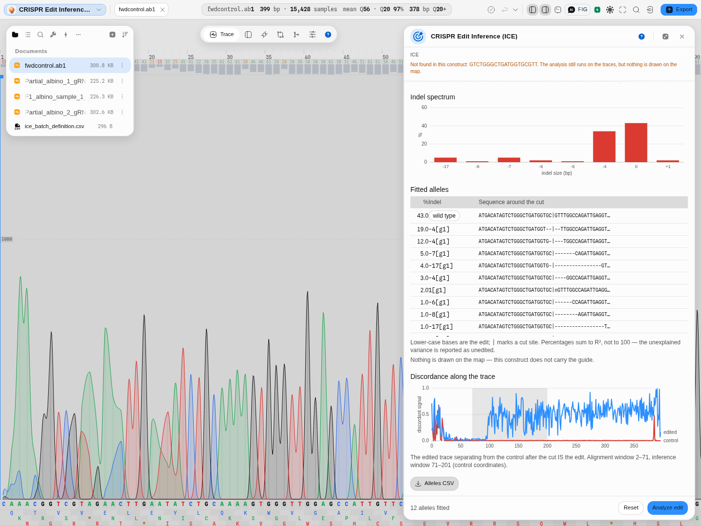
One run, both halves of the argument, because in the panel they sit one above the other.
The spectrum, above: a real edited amplicon against its wild-type control, twelve alleles fitted, 43% of the signal unedited, and the rest spread from −17 to +1. The x axis is a set of named bins, not a coordinate — a −4 and a −17 sit side by side however far apart those numbers are.
The evidence, below: per-base discordance between the two traces, with the inference window shaded. The edited read agrees with the control up to the cut and separates after it, and that separation IS the edit. A read that diverges BEFORE the cut is telling you something other than editing — a mixed template, or the wrong reference — which is why this plot sits next to the numbers rather than behind them.
Limitations
- A control is mandatory, from the same amplicon, in the same direction. There is no reference-free mode, and there should not be: without a control the peak heights have nothing to be relative to.
- Sanger sees a population, not chromosomes. Two alleles reported at 20% each may be two chromosomes at 20% or one at 40% in half the cells. Clonal genotyping needs cloning or amplicon sequencing.
- Large lesions are invisible. A deletion that removes a primer site simply does not amplify, so the pool it came from is missing from the read entirely and the reported edit rate is biased downward. This is a property of the assay, not of the software.
- The fit degrades with trace quality. A poor R² is reported, never hidden — read it before reading anything else. There is no threshold to read it against, from either method's authors: what the reading does instead is tell you how much of your own trace the fit failed to explain, in the same units as the edit rate it reports.
- TIDE takes one guide and one break. Its decomposition is defined around a single cut site, and upstream requires a guide of exactly 20 nt. For a multiplexed edit, ICE above handles all the guides together; the panel says which guide TIDE ran on.
- TIDE reports indel SIZES, not alleles. Two different four-base deletions are one −4 class to it. That is the trade for the p-values, and it is why the two methods sit side by side.
- A base edit right beside the cut is ambiguous. A one-base deletion or a templated repair next to the break can look like a substitution in the trace. On Cas9 nuclease reads (where no base editor was used) the fit finds substitutions of 5% or more only within five bases of the cut, so every base edit that close is reported with a note saying an indel could explain it.
- Alleles in one inseparable group have a measured sum and an unmeasured split. Read the group's share, not the individual shares inside it.
- Machine-learning outcome prediction is not offered. Predicting which indels a guide will produce needs trained models we do not have a runnable, citable source for, and a plausible-looking guess is worse than an honest absence.
Compared with other tools
The published web tools for this — Synthego's ICE, TIDE, and CRISPResso for sequencing reads — each run in a browser you upload to. What is different here:
- Nothing is uploaded. The traces stay on your machine; the decomposition runs locally.
- A plate is one press with an editable plan, and the pairing is shown before the run rather than inferred from a naming convention.
- It sits inside the editor, so the guide can come from a selection on a real construct, and the verification primers, the guide design and the trace editor are the same workspace rather than three sites.
- Both published Sanger methods, on one pair of files. ICE and TIDE are separate web tools you would otherwise upload the same two traces to twice, and read side by side yourself. Here they are one panel, and their disagreement is visible rather than something you have to go looking for.
- The knobs are on the panel. TIDE's read window, indel range, decomposition window and significance threshold are controls next to the result, not defaults you have to accept.
- What they have that we do not: TIDER, the template-directed variant of TIDE, quantifies an HDR knock-in against a designed template — ICE's donor mode answers a related question but is not the same method. CRISPResso works from next-generation reads rather than Sanger, which is a different assay entirely.
Export
The allele table and the batch results table each export as CSV, with the dropped samples and their reasons included in the batch file. TIDE's indel table exports separately — one row per indel size with its percentage, its p-value and whether it cleared your threshold. The consensus edited sequence and per-allele sequences are in the table for copying.
Provenance
Each run records which two files it used, the guide, the maximum indel size and the donor, so a number in a report can be traced back to the exact reads it came from. The sample corpus that ships with the tool names its source deposit, licence and retrieval date, and the published values for each trace — which is what lets you check the tool against a known answer before you trust it on your own data.
Both methods are independent implementations of their published descriptions, checked against Synthego ICE 1.2.0 and the TIDE authors' own code on every trace in that corpus, and against mixtures whose composition was set in advance, where the right answer is known rather than agreed.
Related
Feeds it: CRISPR Guide Design (the guide, and the primers that amplify the locus) · Sanger trace editor (inspect or trim a read first). Follows it: Compare to Reference for per-base variant calls across many reads.
In this group: Codon Optimization · Back-translate: protein → DNA, codon-usage weighted or degenerate · CRISPR Guide Design · Genetic Circuit · In-Situ Probes · RBS & Operon Design · Barcode & Index Design · Auto-Annotate · Apply features from a file · Power and sample size: replicates needed to detect an effect, or the power a design has · Trade-offs: which candidates in a table are not beaten on every objective at once
In-Situ Probes
Design a hybridization probe against a transcript or a locus, padlock probes for in-situ sequencing, or HCR v3.0 split-initiator probe pairs: tile, screen for off-target binding, and pick what images.
RBS & Operon Design
Work on the translation-initiation side of an expression construct: read the strength of an existing ribosome binding site, design a 5-prime UTR towards a strength you want, or stack several coding sequences into one operon.