
RBS & Operon Design
Marked experimental: the surface can change.
Work on the translation-initiation side of an expression construct: read the strength of an existing ribosome binding site, design a 5-prime UTR towards a strength you want, or stack several coding sequences into one operon.
| Reached by | Tools → RBS & Operon Design |
| Sample project | RBS & operon design |
What it does
Translation initiation in bacteria is a hybridisation: the 3′ tail of the 16S rRNA in the small ribosomal subunit pairs with a Shine-Dalgarno sequence in your 5′UTR, and how well that pairing happens — against how hard the mRNA is folded over the same region, and how far the SD sits from the start codon — is most of what decides how much protein you get from a given promoter.
This panel works on that side of an expression construct in three ways. Analyse reads the initiation strength of a coding sequence's existing 5′UTR and shows you the parts the number is made of. Design goes the other way: give it a strength you want and it searches Shine-Dalgarno variants and spacer lengths for a 5′UTR that lands there. Operon stacks several coding sequences into one transcript and re-designs each RBS against the real upstream sequence it will actually have, which is the part a per-gene design cannot do.
When you’d use this
Used in: Optimize a coding sequence for expression in another host
Your construct expresses badly and you want to know whether the ribosome binding site is why. Analyse the site in front of your coding sequence and read the three energies separately. A weak Shine-Dalgarno and a strong one buried under a hairpin are different problems with different fixes, and a single strength number cannot tell you which you have.
You are building an expression construct and need a 5′UTR. Design one to a strength you name, insert it, and the design arrives annotated — Shine-Dalgarno, spacer and start codon as separate features — so the thing you ordered is the thing you can read back later.
You are putting several genes in one transcript. Design each ribosome binding site in the operon, not one at a time: the sequence upstream of gene 2 does not exist until gene 1 is placed, so a site designed in isolation is designed against the wrong context.
You are comparing two designs and want a reason, not a ranking. The three terms are shown separately, so "design B is better" becomes "design B has 2 kcal/mol less structure over the same site".
The route through the workbench: pick or design your coding sequence → RBS & Operon Design for the initiation site → Codon Optimization if the first codons themselves need to change → assemble. Coming the other way, if you already have a construct, start by analysing what is in it.
What this computes
Translation initiation as a hybridisation — the 16S rRNA 3′ tail pairing with a Shine-Dalgarno sequence in your 5′UTR — with every part of the number shown separately rather than folded into one score.
Analyse — for an existing 5′UTR: the relative initiation strength, and the terms it is made of: ΔG total, ΔG mRNA (how hard the message is folded over the same region), ΔG hybrid (the SD
pairing itself), the spacing between the SD and the start codon in nucleotides, and how much of the folding window the structure occupies.Design — the other direction: given a strength you want, it searches Shine-Dalgarno variants and spacer lengths for a 5′UTR that lands there, and reports each candidate with the same terms, so you choose on the parts rather than on one number.
Operon — several coding sequences in one transcript, each RBS re-designed against the real upstream sequence it will actually have. That is the case a per-gene design cannot do, because the sequence upstream of the second gene does not exist until the first one is placed.
Promoters — the transcriptional half, beside the two translational ones: a scan for σ70 promoters anywhere in the sequence, reporting for each one its free energy of binding and escape, the transcription rate that energy implies, and the six motifs the energy is made of — the UP element, the −35 hexamer, the spacer, the extended −10, the −10 hexamer and the discriminator — each with its own contribution, plus the R-loop strength of the first transcribed bases. It answers the question the Operon tab raises: that tab places a promoter, and this one finds the ones nobody placed.
The promoter number is a free energy, and more negative is stronger. It is not a score and not a percentage, which is the single most common way to misread it.
Terminators — the other end of the transcript: a scan for intrinsic (rho-independent) terminators, on either strand, reporting for each one a hairpin score, a tail score, the stem length, the stem-loop sequence and the tail sequence it folds into, with its coordinates and strand. Both numbers are lower is stronger, and neither is a free energy — they are costs in the terminator model's own scheme, so they must not be read beside the promoter tab's ΔG as one scale. The question it answers is the one every insert raises: a cryptic terminator you did not put there is the usual reason a downstream gene in an operon goes quiet.
It finds rho-INDEPENDENT terminators only. Rho-dependent termination needs the Rho protein to catch up with the polymerase; it is not a sequence motif, and no scan of this kind can see it.
Every candidate clearing both published cutoffs is listed, and none of them is a call. A hairpin alone does not terminate — the thymine-rich tail after it is what lets the polymerase let go — so both cutoffs must be met at once, and what comes back is ranked rather than decided. No confidence percentage is reported, deliberately: the published one is a lookup into a calibration table that is not ours to redistribute, and approximating it would be a number with no authority behind it.
What it does not compute: protein yield. Initiation strength is one term in expression, and mRNA stability, growth conditions and the protein itself are not in this model. Nor does the promoter scan say a promoter is USED — it sees sequence alone, so repressors, activators, supercoiling and growth phase are all outside it, and it has no significance cutoff to offer: it ranks configurations rather than calling them, because no cutoff has been published for this model. The terminator scan is the same in both respects: it is intrinsic termination only — rho-dependent terminators, antitermination and riboswitches are invisible to it — and it ranks rather than calls.
Where it lives
Tools → RBS & Operon Design, with four tabs: RBS for a single initiation site, Operon for several in one transcript, and Promoters and Terminators for the two ends of the transcript that carries them. Pick a coding sequence with the Target CDS control, or select a region on the canvas and use that.
Show the initiation window on the map draws the folded window and the located Shine-Dalgarno on the sequence. It is highlights only — the project is never modified, and they clear when the panel closes.
Inputs and outputs
In: a coding sequence — a CDS feature on the open record, or a region you select — together with the bases upstream of it, which are the 5′UTR the calculation is actually about. Nucleotide only.
Out, for analysis: the relative strength, the three ΔG terms it is made of, the SD-to-start spacing found, and the folded initiation window as a base-pair arc diagram.
Out, for design: a 5′UTR sequence, with the Shine-Dalgarno variant and spacer it was built from and the strength it achieves.
Out, for an operon: the assembled transcript with each gene's re-designed RBS in place.
Limits are real and stated rather than silent: strength is computed for sequences up to 100,000 nt and design accepts a coding sequence up to 50,000 nt.
Demo
No screencast yet. The worked example above is the whole run in six numbers, and the sample project it uses is one click from the lobby, so the fastest demonstration is to open it and press Analyze strength yourself.
Worked example
Open the RBS & operon design sample — the E. coli lac operon, the construct everyone learned this on — pick lacZ as the target CDS, and press Analyze strength:
| Readout | Value |
|---|---|
| Relative strength | 0.11 |
| ΔG total | 4.91 kcal/mol |
| ΔG mRNA | −10.4 kcal/mol |
| ΔG hybrid | −4.3 kcal/mol |
| SD → start spacing | 5 nt |
Read them together rather than one at a time. The spacing is optimal — 5 nt is exactly the distance the model treats as unpenalised — and the SD
duplex at −4.3 is real pairing. What holds the strength down to 0.11 is ΔG mRNA at −10.4: the initiation window is folded, and the ribosome has to pay to open it. The arc diagram under the numbers is that folding drawn — 19 base pairs, 54 % of the 70 nt window — so a stem reaching across the Shine-Dalgarno is something you see rather than infer.That is also the honest reading of lacZ: it is a natural, regulated RBS, not an expression-optimised one, and a strength of 0.11 relative to a strong designed site is what a natural one looks like.
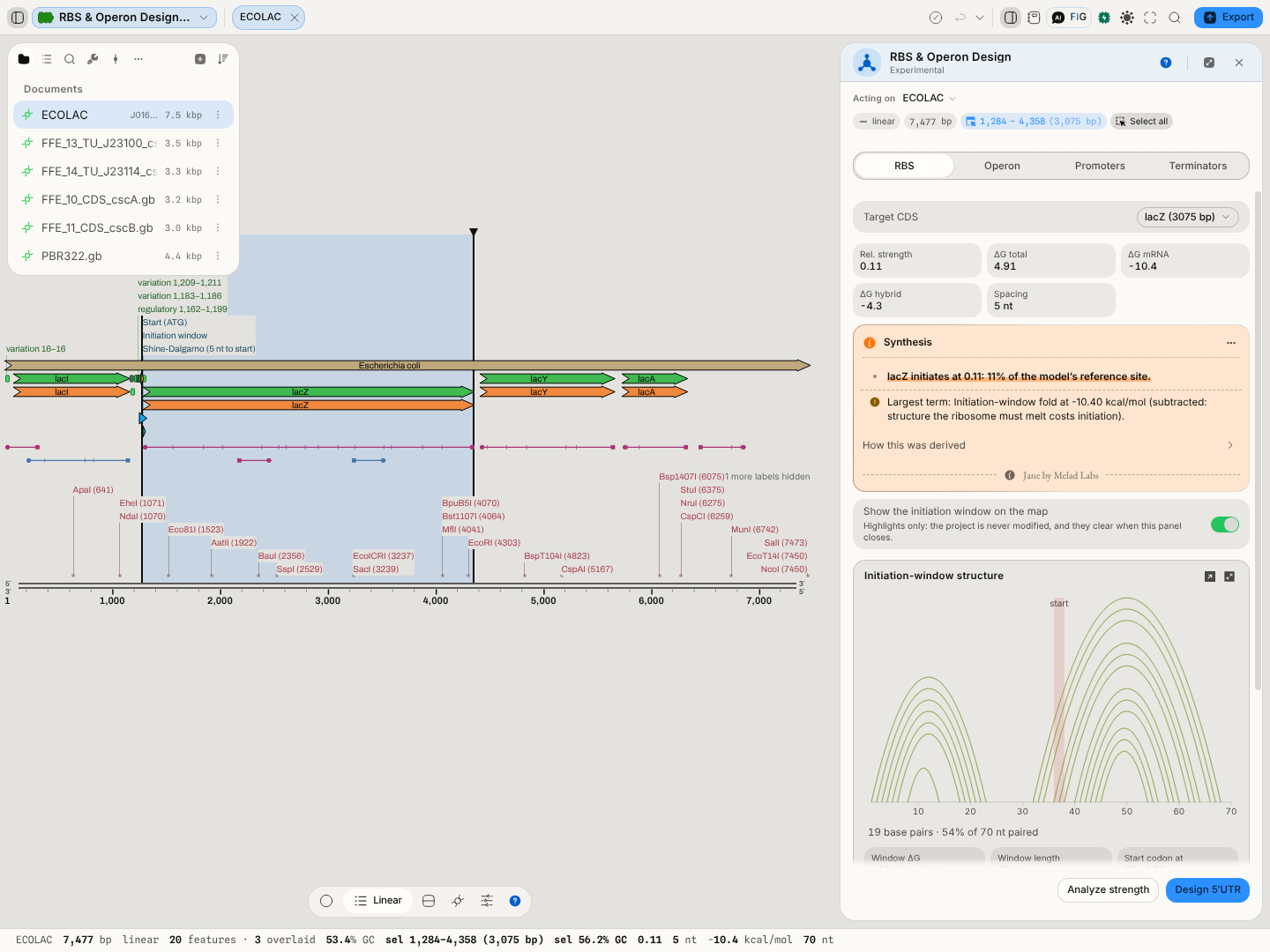 The same run as the worked example, with Show the initiation window on the map switched
on: the start codon, the folded window and the Shine-Dalgarno the model actually paired against are
all marked on the sequence, and the derivation under the readouts shows the four terms the total is
made of.
Controls
| Control | What it changes |
|---|---|
| RBS / Operon | One initiation site, or several coding sequences assembled into one transcript with each RBS re-designed in its real context |
| Target CDS | Which coding sequence the 5′UTR is being read for. Every readout is relative to this gene's start codon |
| Show the initiation window on the map | Draws the folded window and the located SD on the sequence. Highlights only — nothing is written to the project |
| Target (design) | The relative strength to design towards. 1.0 is the model's strong reference; ask for less and you get a weaker SD or a worse spacer, deliberately |
| Analyze strength | Runs the analysis on the current target |
| Design 5′UTR | Runs the reverse design towards the target strength |
Algorithms you can choose
One model, and that is the honest answer here. This is a single published thermodynamic model of translation initiation, not a menu — offering a second one would mean offering a choice between a number you can compare against the literature and one you cannot.
What is yours to change is the question rather than the method: analyse an existing site, design one to a strength you name, or assemble an operon in which every site is designed against its real context. The three run the same energy model.
Bring your own: the Python and R consoles mount the project's files, so an RBS calculator you already trust runs over the same sequence in the same browser tab.
The science
Relative strength is a Boltzmann factor over a total free energy: strength ∝ exp(−β·ΔG_total), with β = 0.45 mol/kcal. ΔG_total is built from four terms, and the panel shows you the three that vary:
- ΔG hybrid — the duplex energy of the Shine-Dalgarno against the E. coli 16S rRNA 3′ tail,
ACCUCCUUA. This is the pairing that recruits the ribosome, and more negative is better. - ΔG mRNA — the folding energy of the mRNA window around the start codon (35 nt each side). This works against initiation: structure the ribosome has to melt is structure it has to pay for.
- A spacing penalty — the SD-to-start distance, scanned over 3–12 nt, penalised by its deviation from the ~5 nt optimum.
- A start-codon term —
AUGat −1.19 kcal/mol,GUGandUUGat −0.075, and the rarer starts lower still, so a non-canonical start is priced rather than ignored.
Design is a coarse-to-fine search, not a formula: a ladder of Shine-Dalgarno variants from
UAAGGAGGU down to no SD at all, crossed with A/U-rich spacers of 4 to 9 nt, with an unstructured
A/U leader prepended so the 5′ end does not fold back over the site being designed. The coarse pass
fixes a spacer and scans the ladder; the fine pass searches around the winner.
The folding is real folding. The mRNA window and the SD
duplex are computed by a Turner-2004 nearest-neighbour folder using ViennaRNA's published parameters, with the same Zuker-style dynamic programming — not a proxy for structure.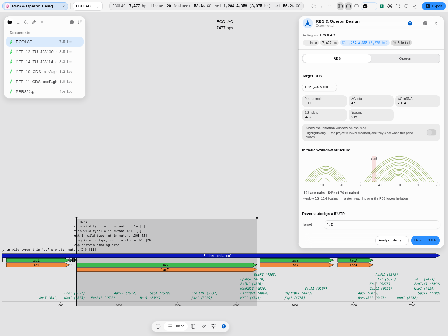
A real run on the E. coli lac operon, lacZ selected. Each arc joins two bases that pair in the folded initiation window, so a stem reaching across the Shine-Dalgarno is something you SEE rather than infer from a number: here 19 base pairs, 54% of the 70 nt window, ΔG mRNA −10.4 kcal/mol, and the start codon marked on the axis. The arcs keep nucleotide i at sequence position i, which is why they can be read against the sequence beneath them.
On correctness. The strength model, the reverse design and the operon assembly are ported algorithm-for-algorithm from the published implementation and checked against it case for case, and the composition with the real folder is checked as its own case — because two separately validated parts do not make a validated whole, and the seam between an energy model and its folder is exactly where a substitution would go unnoticed.
σ70 promoter scan
The promoter model is La Fleur, Hossain & Salis (2022) — a free-energy model over the six motifs above, fitted on 22,132 characterised promoters and validated against measured transcription rates. Correctness here is provenanced by authority rather than by our own testing: every energy is checked against the authors' own implementation, at every transcription start site of every sequence bundled with this app.
It is σ70 — the housekeeping sigma factor of E. coli. It says nothing about σ38, σ32 or σ54 promoters, and nothing about another organism's RNA polymerase. A eukaryotic sequence will still return numbers, because every position scores; those numbers mean "this looks like a bacterial promoter to a bacterial model", which is occasionally what you want to know and never a statement about transcription in a eukaryote.
Intrinsic terminator scan
The terminator model is Kingsford, Ayanbule & Salzberg (2007), the model behind TransTermHP. A hairpin is scored by the paper's own recursion over its pair costs and loop penalties; the tail is scored by d'Aubenton Carafa, Brody & Thermes (1990)'s decay, which weights the thymines nearest the hairpin most. Correctness is provenanced by authority: every candidate is checked against TransTermHP itself, over every circular plasmid bundled with this app, at the precision that program prints.
It reports more than TransTermHP does for the same sequence, and that is a difference in reporting rather than in scoring. TransTermHP keeps one terminator per position after its own overlap filters; this scan returns every candidate that clears both published cutoffs and leaves the choice to you, which is why a strong terminator appears several times at slightly different stem lengths — those are the same structure seen at different extents, not several terminators.
Limitations
- The strength is relative, not a protein yield. It is a number on the model's own scale, useful for ranking designs against each other and for comparing a design against a known site. It does not predict molecules per cell, and no calibration to your strain, medium or plasmid copy number is applied.
- The anti-Shine-Dalgarno tail is E. coli's. The model is parameterised for E. coli translation initiation; a different organism has a different 16S tail and different ribosome, and the number will not transfer.
- Structure is computed over a window, not the whole transcript. A long-range interaction that reaches into the initiation region from outside ±35 nt is invisible to it.
- Design optimises the 5′UTR, not the first codons. The start of a coding sequence contributes to the folding the ribosome must melt, and this tool will not change your CDS to help — Codon Optimization is where that lives.
- An operon's re-designed sites depend on the order you put the genes in, because each is designed against its real upstream. Reordering the genes is a different design, not the same one rearranged.
Compared with other tools
Left deliberately unwritten rather than filled with a comparison table we cannot source: the rule for this section is that every row carries a first-party source and a retrieval date, and the RBS prediction field's incumbents have not been surveyed to that standard here yet. What can be said without one: this panel's distinguishing property is that the three ΔG terms are shown separately alongside the folded window, so a low strength is attributable rather than merely reported.
Export
The designed 5′UTR and the assembled operon leave as sequence, to the clipboard or into the project as a new record. The initiation-window arc diagram is a plot like any other in the workbench and copies or saves as an image.
API
All three operations are available headlessly, so the same numbers can be produced without the panel: scoring the site already in front of a start codon, designing a 5′UTR to a target strength, and assembling an operon. The RNA folder the energy model needs is supplied to them rather than assumed, which is what lets the folding be checked independently of the initiation model.
Separately, the editor's Python and R consoles see the open record — the sequence, the selection and the project's files are bound in both languages — so an RBS calculation written against another library can be run over exactly what is on screen and its output saved back into the project.
Automation
The scientific copilot can call all three by name: score_rbs reads an existing 5′UTR,
design_rbs writes a new one to a target strength, and assemble_operon stacks several
coding sequences and designs a fresh site in front of each against its real upstream context —
which is why the site it gives gene 2 is not the one design_rbs would give that gene in isolation.
It returns the assembled sequence, its layout, and each gene's achieved strength.
Provenance
A run records which coding sequence it was read for, the strength it reported and the three ΔG terms behind it, and — for a design — the target strength, the Shine-Dalgarno variant and the spacer chosen. Nothing is stochastic, so a replay reproduces the same numbers.
Citing the method in a paper means naming the initiation model this implements and the folding parameters underneath it: a Salis-style Shine-Dalgarno ∙ anti-Shine-Dalgarno hybridisation model over the E. coli 16S 3′ tail, with mRNA structure from a Turner-2004 nearest-neighbour folder using ViennaRNA's published parameters.
Screenshots
Both frames on this page sit in the section they illustrate: the panel under Worked example, the arc diagram of the folded window under The science.
Related
What feeds it: a coding sequence — from Back-translate if you started from a protein, or straight from a record you already have.
What follows it: Codon Optimization, when the folding that holds initiation down comes from the first codons of the coding sequence rather than from the 5′UTR — this tool will not change your coding sequence, and that one will.
What it is an alternative to: picking a ribosome binding site from a parts registry. A catalogue part carries a strength measured in someone else's context; this computes one in yours. Both are reasonable, and they answer different questions.
In this group: Codon Optimization · Back-translate: protein → DNA, codon-usage weighted or degenerate · CRISPR Guide Design · Genetic Circuit · In-Situ Probes · CRISPR Edit Inference · Barcode & Index Design · Auto-Annotate · Apply features from a file · Power and sample size: replicates needed to detect an effect, or the power a design has · Trade-offs: which candidates in a table are not beaten on every objective at once