
GC content distribution
How GC content is spread across the barcode set, binned to whole percent, with the mean, spread and range stated on the section header.
What it does
Each bar is a whole-percent GC value; its height is how many barcodes in the set read that value. The header above the plot carries the summary the bars cannot show precisely — mean GC, standard deviation, and the minimum and maximum in the set.
GC content matters for a barcode for reasons that have nothing to do with distance. Barcodes are short, they are synthesised as part of an adapter or a primer tail, and they are read in the first cycles of a run: an extreme-GC member anneals differently from the rest of the pool, amplifies differently, and can be under-represented in the final library while its sequence remains perfectly distinguishable.
A tight distribution near 50% is what a designer usually wants. A bimodal one — two clusters with a gap — usually means the set was assembled from two sources.
When you'd use this
- Before ordering oligos. A member at 20% or 80% GC is the one whose adapter under-performs, and the fix is to swap it while the set is still on screen.
- After importing a set whose GC filter settings you do not know. The panel's own designs can be GC-filtered on generation; an imported set has whatever it has.
- When one sample keeps coming back under-represented across runs and the barcodes are otherwise well separated — GC spread is the first place to look.
- When mixing two kits into one pool, where the combined distribution is the thing nobody has looked at.
What this computes
- GC content per barcode, as the fraction of G and C bases, by the same routine the rest of the workbench uses for GC — one implementation, so this number and the number on a sequence map cannot disagree
- Counts per whole-percent GC bin. Whole percent deliberately: at barcode lengths of 6 to 12 bases only a few GC fractions are achievable at all (an 8-mer can only be 0, 12.5, 25 … percent), so finer bins would draw a comb of empty space between spikes and imply a resolution the data does not have
- Mean, standard deviation, minimum and maximum, computed over the whole set rather than over the bins, so they are exact rather than binned estimates
- A flag per barcode falling outside the design GC window, in the set browser beside the value
Mixed-length sets are fine here, unlike the per-cycle plots: GC content is a fraction, so it is comparable across lengths.
Where it lives
The Analysis tab of the Barcode & Index Design panel, below the two distance histograms. The section header shows mean, standard deviation and range, and carries the detach control that floats the plot as a live surface beside the canvas.
Inputs and outputs
In: the panel's working set. Mixed-length sets are fine here — GC content is a fraction, so it is comparable across lengths, unlike the per-cycle plots which need equal lengths and say so when they do not get them.
Out: counts per whole-percent GC bin, plus the mean, standard deviation, minimum and maximum in the header. Per-barcode GC is also a sortable column in the set browser, and barcodes outside the design GC window carry a flag there.
Screenshots
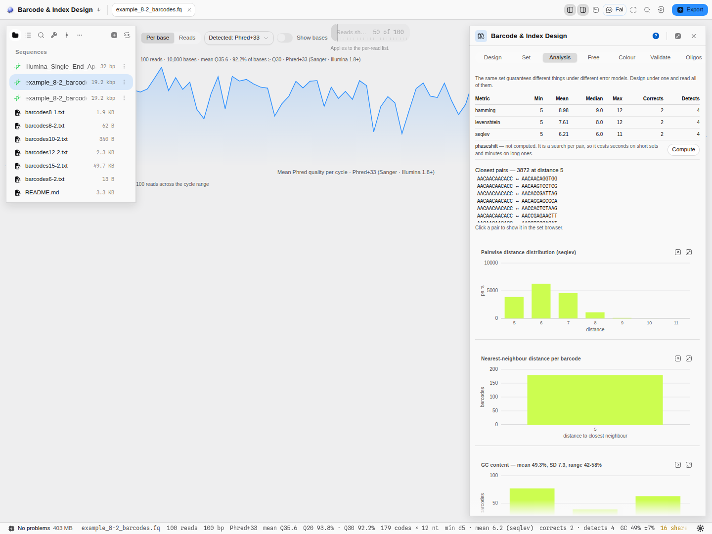
Controls
| Control | What it changes |
|---|---|
| GC filter (Design tab) | Whether newly designed barcodes are constrained to a GC window at all. It shapes what a design run produces; it does not filter what this plot draws, which is always the whole working set. |
| The working set | Editing it redraws the distribution. |
| Detach | Floats the plot beside the canvas. |
The science
GC content is computed per barcode as the fraction of G and C bases, by the same routine the rest of the workbench uses for GC — one implementation, so the number here and the number on a sequence map cannot disagree.
Binning is to whole percent, deliberately: at barcode lengths of 6 to 12 bases only a few GC fractions are even achievable (an 8-mer can only be 0, 12.5, 25 … percent GC), so finer bins would draw a comb of empty space between spikes and imply a resolution the data does not have.
The mean and standard deviation in the header are computed over the whole set, not over the bins, so they are exact rather than binned estimates.
Limitations
- GC content is a composition summary and nothing more. It cannot see where in the barcode the GC sits, and a barcode with all its Gs in a row is a synthesis and phasing risk that this plot cannot distinguish from a well-mixed one. The longest-run column in the set browser is the readout for that.
- It says nothing about distance. A set can be perfectly balanced for GC and undecodable.
- Whole-percent binning means two barcodes of different lengths with slightly different fractions can share a bar.
Related
In this group: Edit annotation · Enzyme · Insert sequence · Merge features · Manage enzymes · Dot plot · Dot plot grid · Melt curve · Amplification curves · Population genetics · RNA-seq · Site avoidance heat map · Protein coverage · Reference-gene stability · Digital PCR · Codon usage matrix · Pairwise distance distribution · Nearest-neighbor distances · Base composition per cycle · Pairwise distance grid · Per-cycle channel occupancy · Grammar assembly plan · Gibson assembly plan · Assembly plan build order · Golden Gate assembly plan · Guide track · Primer binding track · Hydropathy profile · Charge vs pH · Amino-acid composition · Hydrophobic moment · Optimization profiles · Digest gel · Virtual gel · Initiation-window fold · Antibody domain map · Electropherogram · Circuit netlist · Circuit transfer functions · Circuit construct · Construction graph · Protocol · Read Quality Profile · Read Alignment · Raw Signal · Verify vs Reference · Chromosomal microarray · Variant calls · Small molecule