
Variant Calls
Open a VCF as a real variant table — typed, filtered and countable — rather than as text you scroll.
| Reached by | Tools → Variant Calls (VCF) |
| Sample project | Variant calls (VCF) |
What it does
A VCF is a tab-separated file with a header, and almost every tool that "supports" it either shows you the raw lines or loads the whole thing into memory to build a table. Neither is useful on a real call set: the file can be gigabytes, and the questions you actually have — how many of these are SNVs, what is the Ts/Tv ratio, what did the caller reject and why, does this sample carry it — are not answerable by reading rows.
This decodes the file into a typed table. Every record is classified by allele type using htslib's own rule, counted, and made filterable along the axes a caller's output is actually interrogated on: type, contig, FILTER, QUAL, multiallelic, INFO field, and per-sample genotype.
And when the file is bgzipped with a .tbi or .csi index, it is read by locus rather than
ingested — the second format in the app to obey "index, never ingest", after BAM.
When you'd use this
Used in: Read a variant call set at a locus
- You ran a variant caller and want to know what it produced before pushing it downstream. The Summary view answers that in one screen: counts by type, Ts/Tv, the substitution matrix, per-contig and per-FILTER breakdowns.
- You are checking an edit. A CRISPR or mutagenesis experiment produces an expected change at a known coordinate; open the calls, jump to the locus, and see whether it is there and what else came with it.
- You are auditing a caller. Filter to a FILTER id rather than past it —
Keep only records carrying this FILTER idis how you look at what the caller threw away, which is the question aPASS-only view can never answer. - You need a region out of a huge call set. With an index, the region control reads only the blocks covering that locus.
- You want the variants on the sequence you have open. Set
Sequence starts atand the records hand off to the map at the right coordinates.
Ts/Tv is the fastest sanity check in the list: for human whole-genome calls it usually sits near 2, and a value far from that is normally an artefact of the calling rather than biology.
What this computes
Every number here is read out of the call set you opened. Nothing is re-called and nothing is
inferred: this reports what the caller wrote down, in the terms bcftools uses for the same file.
Per record
- Allele type — SNV, indel, MNV, symbolic/SV, breakend, spanning deletion — from htslib's
bcf_set_variant_type, ported faithfully, as a per-allele mask rather than a single label, so a site can be both an SNV and an indel and is reported as both - QUAL, FILTER, INFO and per-sample FORMAT fields as written, with floating-point values
re-printed in the form
bcftoolsitself produces, digit for digit - Missing distinguished from end-of-vector, so a haploid chrY call reads as haploid rather than as missing data
Per call set (the bcftools stats sections)
- SN counts, the transition/transversion ratio — offered two ways, over all ALTs and over the first ALT only, because the field genuinely uses both — the substitution matrix, the indel-length distribution, per-contig totals, and the FILTER and QUAL breakdowns
Per sample
- Hom-ref, het, hom-alt, singleton and missing counts
Filtering happens in the engine, not in the table, so the table, the exports and the map track can never disagree about which records you are looking at. Two controls that look alike are not: Region re-reads the file through the index (and is inert, and says so, without one), while Positions narrows the records already in hand, needs no index, and — because it holds them — names back a contig your file does not have instead of returning an empty table.
Coordinates are yours to set. Sequence starts at is the contig coordinate of the open sequence's first base; leave it at 1 when the sequence is the contig, and set it when what is open is a slice — a plasmid, an amplicon, a gene — or every hand-off to the map lands the width of that slice away.
Out: a filtered VCF, a filtered BCF, a TSV of the table, and a BED of the record intervals.
Where it lives
Tools → Variant Calls (VCF) opens a file picker and the call set becomes its own stage tab —
a document rather than something you load into a viewer. A .vcf already in the project opens from
the file manager, and a bgzipped .vcf.gz is grouped with its .tbi/.csi automatically.
Beside the table, while a call set is the document you are looking at, the Variant calls panel reads it back to you: what the records add up to, how each figure was derived, which filters are narrowing what you see, and what about the file the numbers cannot be taken to mean.
It is part of the editor rather than a viewer beside it:
- Clicking a row selects that variant on the focused sequence editor. A position outside the open sequence is refused rather than clamped — clamping would put a mark somewhere plausible and wrong, which is the failure you would never notice.
- A variant can be applied to the sequence, and the REF is checked against the bases first: a mismatch refuses and names what it found there instead.
- The same component draws the stage tab and the file-manager preview, so the two cannot drift.
Inputs and outputs
In: a VCF (4.x), plain or bgzipped, or a BCF — the binary encoding of the same data. An
index (.tbi/.csi) is optional for a VCF, unlike a BAM's, where it is required, because an
unindexed VCF still reads whole. Without one, the region control simply has nothing to drive.
A BCF opens as the same table, with the same three views, the same filters and the same exports. Nothing about the workflow changes; the only difference you will see is that the region control is switched off (see Limitations).
Out: the variant table, the summary statistics, per-sample genotype counts, and four exports —
a filtered VCF, a filtered BCF (the binary encoding, for handing to bcftools or any
htslib-based tool), a TSV of the table, and a BED of the record intervals.
What it refuses, and what it says: a .tbi/.csi selected on its own is refused by name — it is
the companion of a call set, not a document — with the instruction to select the .vcf.gz it belongs
to.
Demo
Not recorded yet. The screencast worth making is the region control on the indexed
volvox.test.vcf.gz: type a locus, watch only that window read.
Worked example
data/samples/VCF/simple.vcf — the VCF 4.3 specification's own worked example, chosen because
its five records are the canonical edge cases and anyone can check this table against the spec.
Three samples: NA00001, NA00002, NA00003. Running it gives:
CHROM  POS      ID          REF  ALT     QUAL  FILTER  TYPE       END
20     14370    rs6054257   G    A       29    PASS    SNP        14370
20     17330    .           T    A       3     q10     SNP        17330
20     1110696  rs6040355   A    G,T     67    PASS    SNP        1110696
20     1230237  .           T    .       47    PASS    ref        1230237
20     1234567  microsat1   GTC  G,GTCT  50    PASS    insertion  1234569
And the Summary view:
records                5        multiallelic sites      2
SNVs                   3        …of which SNV-only      1
indels                 1        records with no ALT     1
Ts / Tv             2 / 2       ratio                 1.00
Ts / Tv (first ALT) 2 / 1       ratio                 2.00
Four things in that output are worth reading carefully, because they are exactly where a VCF viewer is usually wrong:
20:1230237has no ALT (.) and is typedref, not dropped. A record asserting no variant here is real VCF and carries information; the countrecords with no ALT = 1keeps it visible rather than silently reducing the file to four rows.20:1234567isGTC → G,GTCT— one deletion and one insertion at the same site. It is labelledinsertionand itsENDis 1234569, not 1234567, because the REF spans three bases. A viewer that treats every record as one base gets the interval wrong here.- Ts/Tv is reported twice, and the two disagree (1.00 vs 2.00). Over all ALT alleles there are 2
transitions and 2 transversions; over first ALTs only, 2 and 1.
20:1110696isA → G,T, andA→Gis a transition whileA→Tis a transversion — so which number you get depends on whether multiallelic sites are counted once or per allele. Both are shown because both are used, and a single number would be a silent choice on the reader's behalf. multiallelic sites = 2butSNV-only multiallelic = 1—20:1110696(G,T) and20:1234567(G,GTCT) are both multiallelic; only the first is all-SNV.
Reproduce it with the API block below, or open the Variant calls (VCF) starter and pick
simple.vcf.
Putting a call on the map
A variant table answers what was called. The next question is always where, and the two hand-offs below are what make a call set part of the molecule rather than a spreadsheet beside it. Both need one thing: the reference the calls were actually made against, open in the editor.
The Variant calls (VCF) starter now ships that pair. It opens on NC_045512.2, the SARS-CoV-2 reference genome (29,903 bases, 11 genes, 26 mature peptides), and carries 104 real calls from NCBI's own variant-calling pipeline over an Illumina amplicon run of a clinical isolate. Every one of those records was called against that exact genome, which is what the two actions below rely on.
Click a row and its bases are selected on the sequence. The selection spans the whole REF allele, not just the base the record is anchored on, so a seven-base deletion selects seven bases. The sequence view scrolls to it, and the readout tells you what you have landed in: for the record at 21,765 it reads codon 68 of S, the spike gene. That is the Δ69/70 deletion, and one click is the whole distance between "a number in a table" and "a lesion in a protein".
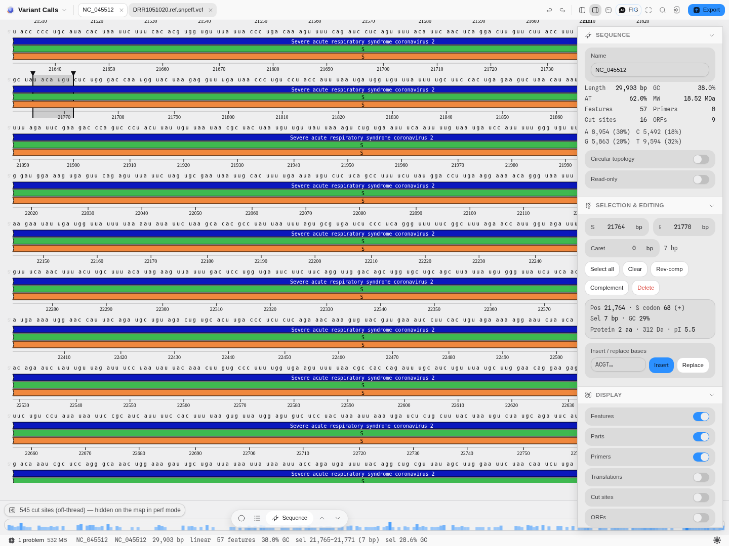
Press Apply and the ALT allele is written into the sequence. This is a real edit: annotations move with the bases, so an indel does not leave every downstream feature pointing at its old coordinate. Applying the 21,765 deletion takes the genome from 29,903 to 29,897 bases and the features that follow it shift by six.
Apply checks the REF against the bases first, and refuses when they disagree. This is the guard that matters most, because a call applied to the wrong reference produces a sequence that looks entirely plausible and is wrong. The starter includes the case deliberately: alongside SARS-CoV-2 it carries NC_004718, the 2003 SARS coronavirus, a different virus of almost the same length. Focus that one, press Apply, and you are told exactly what was found where:
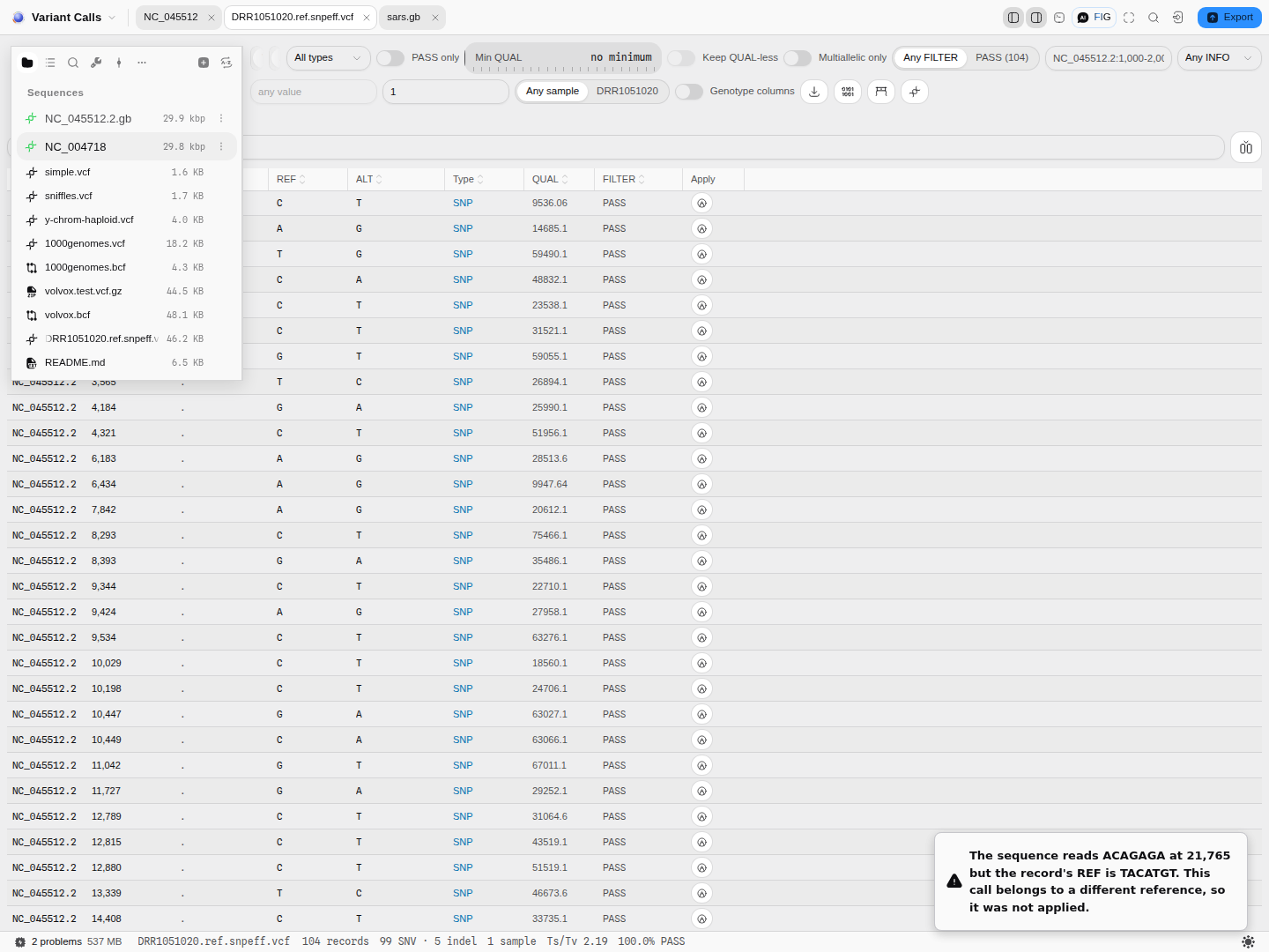
One thing the check deliberately does not refuse: an RNA reference read with U where the
call set writes T. Variant callers report against a DNA reference even for an RNA virus, while
the record you open declares itself RNA and is displayed as RNA, so those two spellings are the same
base and are treated as such. Ambiguity codes are not folded in the same way: an N in a reference
does not tell you the base is the one the record claims, so it still refuses.
If what you have open is a slice of the contig (a gene, an amplicon, a plasmid carved out of a genome), set Sequence starts at to that slice's first coordinate in the contig. Both hand-offs read it, and the REF check is what catches it being wrong, which is the point of stating it rather than guessing.
Controls
Region — a locus (chr:start-end). Re-reads the file through the index, so it is the control
that makes a large call set usable. Needs a .tbi/.csi; without one it is inert and says so.
Positions — narrows the records already read. Unlike Region it needs no index and never
re-reads: it filters what is in hand. Because it already holds the records, it also knows which
contigs the file has, so on a single-contig file a bare range is enough (21,700-21,800); on a
file with several it asks you which contig you mean, by name, rather than returning an empty table.
A contig the file does not have is named back to you the same way. The two look similar and are not, which is why they are named
differently.
View — Variants (the table) · Summary (the bcftools stats sections: SN counts, Ts/Tv, the
substitution matrix, indel-length distribution, per-contig totals, FILTER and QUAL breakdowns) ·
Samples (per-sample hom-ref, het, hom-alt, singletons, missing).
Filters run in the engine, not in the table. That is why the table, the exports and the map track can never disagree about which records you are looking at.
| Control | What changing it does |
|---|---|
| Contig | Restrict to one contig. The list is the contigs actually present, with counts |
| Type | All · SNVs · Indels · MNVs · Symbolic/SV · Breakends · Spanning deletions. A site can be both an SNV and an indel — types come from htslib's per-allele mask, not a single label |
| PASS only | Hide records carrying any FILTER other than PASS |
| Min QUAL | Floor on QUAL. Records with no QUAL are hidden once a minimum is set, because there is nothing to compare |
| Keep QUAL-less | Puts those records back. Without it, a caller that never writes QUAL appears to have no variants at all — which looks like a broken file and is not |
| Multiallelic only | Records with more than one ALT |
| FILTER | Keep only records carrying one specific FILTER id. This is how you inspect what a caller rejected |
| INFO field / INFO contains | Keep records where a field is present; optionally substring-match its value, case-insensitively. A flag field (DB, SOMATIC) needs no value |
| Carried by | Keep records where one named sample has a non-reference genotype |
| Genotype columns | Which sample columns to draw. On a 1,233-sample cohort this is the difference between a readable table and an unusable one |
| Sequence starts at | The contig coordinate of the open sequence's first base. Leave at 1 when the sequence is the contig; set it when what is open is a slice — a plasmid, an amplicon, a gene — or every hand-off to the map lands the width of that slice away |
Algorithms you can choose
Deliberately few, and that is the honest answer: variant typing is not a matter of taste, it is a matter of agreeing with the tool the reader will check against.
- Allele typing is htslib's
bcf_set_variant_type, ported faithfully, and there is no alternative offered. This matters: PyVCF3 has avar_typetoo, and it classifies differently. Using it would have made every SNV/indel/Ts-Tv number on this page disagree with thebcftoolsoutput a reader compares against — so the rung of the source ladder was chosen for agreement, not convenience. - Ts/Tv is offered two ways (all ALTs, and first ALT only) because the field genuinely uses both. See the worked example.
Bring your own: the Python and R consoles mount the project's files, so pysam/cyvcf2 or
VariantAnnotation run over the same file in the same tab; @ports/vcf is callable directly; and
the filtered VCF export means any downstream tool can pick up where the table left off.
VCF and BCF: the same data, two encodings
BCF is not a different format — it is the same records written in binary. A caller emits VCF text;
bcftools view -O b writes the identical content as BCF. Files shrink, and a machine reads them
without re-parsing text.
Three consequences are worth knowing when you open one:
- Every tag becomes a number. BCF stores a dictionary in its header and replaces every contig, FILTER, INFO and FORMAT name with an index into it. That is why the header must declare everything a record uses, and why a header-less VCF has no BCF form at all.
- Numbers are stored as numbers. A
QUALof100is four bytes, not the characters1,0,0. Floating-point values are therefore re-printed when you read them back, and the printed form here is the onebcftoolsitself produces, digit for digit, so a value you compare againstbcftools viewoutput will match. - Missing and "end of vector" are different things. A genotype field wide enough for diploid samples has to carry haploid ones too, so BCF marks where a shorter genotype ends. This is why a haploid chrY call set reads as haploid here rather than as missing data — the same distinction the per-sample counts make for text VCF.
Open the sample project's 1000genomes.bcf next to its 1000genomes.vcf: same 2 records, same
1,233 samples, same Ts/Tv. If they ever disagreed, one of the two readers would be wrong, which is
exactly why the sample project ships both.
The science
VCF is a specification, not an algorithm, so the work is in obeying it exactly:
- Parsing is
@gmod/vcf, a spec-tracking parser. For a file format, a maintained parser is the right rung of the ladder — it handles a decade of real-world malformity that a hand-rolled reader would not. - Allele typing is a faithful port of htslib's
bcf_set_variant_type, which produces a per-ALT bit mask,ORed into the record'sd->var_type. That is why a record can be both an SNV and an indel, and why the type filter is a mask test rather than a string comparison. - Statistics are a port of
bcftools' ownvcfstats.c— SN counts, Ts/Tv, the substitution matrix, the indel-length distribution, per-contig totals and the FILTER/QUAL breakdowns. No npm package defines those the way bcftools does, and a different definition would make every number disagree with the output a reader checks against. - Indexed reads go through
@gmod/tabix: the binning index over BGZF blocks, the same mechanism the BAM reader uses.
199 tests stand behind it: byte-for-byte against the real htslib C, the indexed path against the
whole-file path, and a cross-check against scikit-allel. The htslib function is self-contained
enough to be extracted and compiled with a small gcc harness, so the vectors are regenerable
without building htslib.
Limitations
- Ts/Tv over all ALTs and over first ALTs disagree on multiallelic sites, and neither is "the" answer. Both are shown. Compare like with like when quoting one.
- An unindexed call set is read whole, up to 128 MB of uncompressed text. There is no streaming
path without an index, so a very large plain
.vcfis bounded by memory and past that ceiling it is refused rather than half-read. The refusal names the fix for what you are holding:tabix -p vcfif the file is already bgzipped,bgzipfirst if it is plain. An INDEXED call set has no such ceiling — over 128 MB it opens at its header and is read one locus at a time, which is the whole reason to index before you need to. - A region's statistics are the region's. Every census in the panel describes the records
actually read, and says so beside them (
19 in region). Where a file was never read whole, the status line saysnot read wholerather than counting zero — a file's own totals are not knowable without reading all of it, and the panel will not guess them. - A BCF export needs a complete header. Writing BCF works (
Export BCF), but BCF has no way to store a contig, INFO or FORMAT tag the header never declared, so a file with an incomplete header is refused by name rather than written with invented declarations. Export it as VCF instead. - A BCF cannot represent every VCF, and that is the format, not this reader. BCF replaces every
tag with an integer into a dictionary built from the header, so a VCF that uses a contig, INFO or
FORMAT tag it never declared — or that has no
##header at all — cannot be encoded as BCF by anything,bcftoolsincluded. Such files still open here as text VCF. Min QUALsilently excludes QUAL-less records unlessKeep QUAL-lessis on. This is deliberate and stated in the control's own hint, but it is the one filter interaction that can make a file look empty.- A header's
##contigdeclarations are not checked against the index, on purpose. That check was written and deleted the same hour:volvox.test.vcf.gzdeclaresID=20/ID=ctgAwhile every record in it is oncontigA, because declaring contigs is optional and unenforced in VCF. The check fired on a correct file, and a guard that false-alarms on real data is worse than no guard. A test pins the finding so it is not re-added. - Genotype-aware statistics are per-sample counts, not population genetics. No allele-frequency estimation, no Hardy-Weinberg, no LD.
Compared with other tools
Sourced from each vendor's own pages, retrieved 2026-08-08 — see the open claim register.
Geneious Prime states next-generation-sequencing analysis including genome visualisation and SNP/variant analysis, alongside de novo assembly and read mapping. It is a desktop application. Its NGS scope is far wider than this tool's — we do not assemble genomes or map reads at all.
SnapGene's published feature list does not include VCF or variant analysis; its sequencing work is Sanger-side (alignment to a reference, and CAP3 contig assembly).
What is different here rather than better: this reads an indexed VCF by locus in a browser tab,
with no install and no upload; it opens BCF, the binary encoding, in the same tab without asking
you to convert it first; and its typing agrees with bcftools by construction. What is genuinely
missing compared with a full NGS suite: everything upstream of the call set.
Export
- Export VCF — the filtered records, with the original header preserved so it round-trips.
- Export BCF — the same records in the binary encoding. Smaller, and read directly by
bcftoolsand anything else built on htslib. Refused, by name, if the header does not declare every contig and tag the records use, because BCF has no way to store an undeclared name. - Export table — TSV of exactly the columns and rows on screen.
- Export BED — the record intervals, using the same
ENDlogic as the table (so theGTC → G,GTCTrecord exports as a 3-base interval, not a point).
Filters apply to all three: what you exported is what you were looking at.
API
import { readVcf } from '@ports/vcf';
import { computeVcfStats } from '@ports/vcf';

const doc = readVcf(await file.text());

doc.header.samples;        // ['NA00001', 'NA00002', 'NA00003']
doc.variants.length;       // 5
doc.variants[4].label;     // 'insertion'
doc.variants[4].end;       // 1234569 — REF spans three bases
doc.variants[4].typeMask;  // 196 — htslib's OR of both ALTs' types

const stats = computeVcfStats(doc);
stats.counts.snps;            // 3
stats.counts.multiallelicSites; // 2
stats.tstv.ratio;             // 1    (all ALTs)
stats.tstv.ratioFirstAlt;     // 2    (first ALT only)
Positions are 1-based, as written in the file; end is inclusive. filters: [] means PASS was
written, which is not the same as the column being .. Reading is pure; indexed region reads are
async because they touch the file.
Automation
The table is a document, so anything that consumes a document consumes it. There is no dedicated
workflow DAG node and no copilot tool for variant filtering — that is a real gap rather than a
design decision, and it means a pipeline cannot currently express "filter to PASS SNVs on chr20".
Calling @ports/vcf directly is the way to do it in code today.
Provenance
The filtered VCF export preserves the original header verbatim, so the file states which caller and which reference produced it — the provenance travels with the data rather than with our record of it.
What the app records is the file and the filters applied; a locus read through the index is a read, not an edit, so it writes no step. Citing the method means citing the caller that produced the file, plus htslib's typing rule for any count taken from this table.
BCF decoding is checked against htslib itself. Every sample call set is encoded to BCF by real
htslib and rendered back to text by it; our reading of the same bytes is required to match that
output line for line, including the exact printed form of every floating-point value. So a number
you read here and a number bcftools view prints for the same file are the same number, not two
independent estimates of it.
Screenshots
The canvas captures canvas/vcf-1000genomes.png, canvas/vcf-haploid-y.png and
canvas/vcf-sniffles-sv.png show the decoded table on a real 1,233-sample cohort and on the haploid
and structural-variant cases; they belong on
the Variant table canvas page.
The Summary view now has a frame — canvas/bcf-summary.png, shot on a BCF, showing the counts,
Ts/Tv, the substitution matrix and the per-contig and FILTER breakdowns in one screen.
canvas/bcf-samples.png covers the per-sample counts with every call haploid.
The filter controls now have a frame too: panel/variants-indel-filter.png shows the type
filter narrowing the SARS-CoV-2 run to 5 of 104 records, every indel it called, with the
per-sample genotype column switched on and each record typed by htslib's own rule.
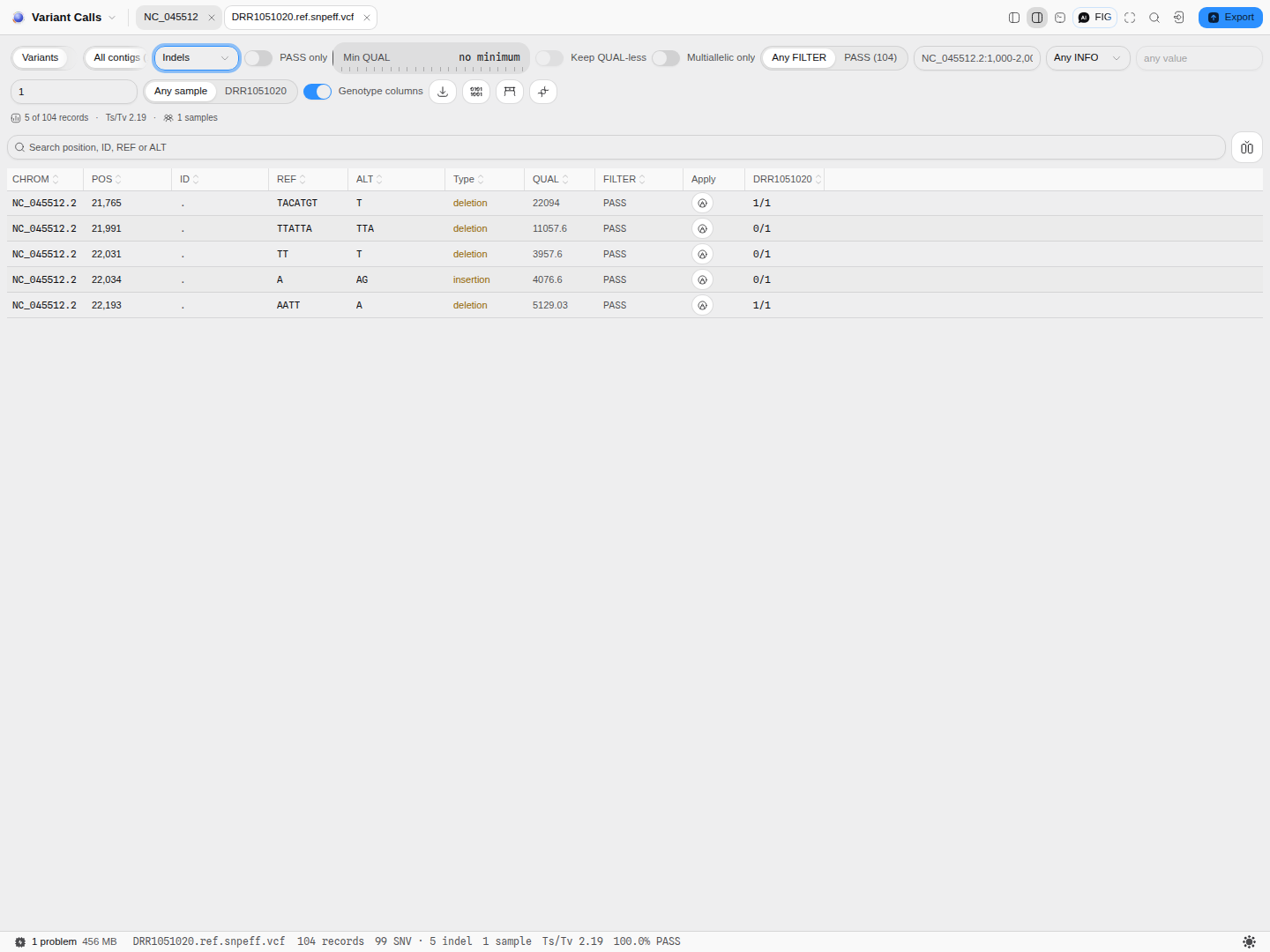
Still missing: a frame of the region control mid-read on an indexed file.
Related
Feeds it: any variant caller's output; the file manager; an indexed .vcf.gz with its .tbi.
Follows it: the sequence map, which draws a record at its coordinates; the Variant table canvas for how the drawing itself is read.
Compare with: Read Alignment (BAM · SAM), the other format read by index rather than ingested — same mechanism, different question.
In this group: Chromatogram · Map reads to a reference · Fragment analysis · Alignment · Population genetics: allele frequencies, Hardy–Weinberg, Fst, linkage disequilibrium · RNA-seq: differential expression with DESeq2, over-represented gene sets, gene set enrichment · Multiple Sequence Alignment · Compare Traces to Reference · Sequencing Verification · Screen for vector contamination
Alignment
Open a sorted, indexed BAM — or a SAM, which needs no index — and look at a locus: the coverage over the window and the reads beneath it, drawn from the real CIGAR so insertions and deletions land where the aligner put them.
Population Genetics
Read a cohort's genotypes by population: allele frequencies, heterozygosity and Hardy–Weinberg tests per site, Fst between populations, linkage disequilibrium between sites, principal components of population structure, and individual ancestry coefficients.