
Amplification Curves → Cq
Fit a model to each amplification curve and read the quantification cycle off the fit — with the definition of "Cq" as an explicit choice, because there is more than one.
| Reached by | Tools → Amplification Curves → Cq |
| Sample project | qPCR & digital PCR |
What it does
A quantification cycle is not a measurement. It is an estimate of where an exponential began, recovered from a curve that has already left the exponential phase by the time you can see it — and the field has at least seven ways of placing it. They are not one estimator with a flag. They are different quantities, and on the same curve they land on different cycles.
On one real reaction from the bundled example run:
| Cq definition | Cycle |
|---|---|
| cpD1 — first-derivative maximum | 17.36 |
| cpD2 — second-derivative maximum | 15.44 |
Same fluorescence readings, same fitted model, 1.9 cycles apart. At an efficiency near 2 that is close to a four-fold difference in inferred starting quantity. Neither number is wrong; they answer different questions, and the real error is comparing a plate analysed with one against a plate analysed with the other.
So this panel fits the curve first and reports the whole fit — coefficients, residual variance, two R², AICc, BIC — and then lets you say which cycle you want off it. The picture is part of the point: you can see whether the sigmoid actually follows the readings, and whether the marker sits on the elbow or somewhere you would not have put it.
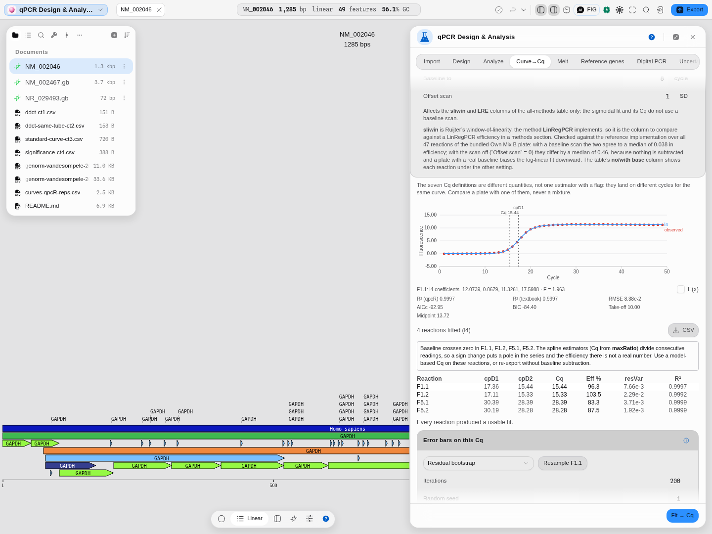
Reaction F1.1 of the example run: observed fluorescence per cycle (points) with the fitted four-parameter log-logistic model through it (line), R² 0.9997. The two dashed verticals are cpD1 and cpD2 on that one curve — the 1.9-cycle spread in the table above, drawn.
What this computes
Per reaction, from its own fluorescence readings
- a fitted sigmoid — four to seven parameters, log-logistic (l4–l7) or logistic on the raw scale (b4–b7) — with its coefficients, and the option to let model selection choose among all eight
- the quantification cycle under any of seven definitions: cpD1 (first-derivative maximum), cpD2 (second-derivative maximum), the cycle of maximum efficiency, an exponential-region point, Cy0, the cycle at 20% of the fluorescence at the Cq, and the model-free maxRatio; or, when you set one, the classic threshold cycle (Ct), where the fitted curve crosses a fluorescence threshold
- the initial fluorescence two ways: the fitted curve at cycle 0, and the fluorescence at the Cq divided by the efficiency raised to the Cq. They agree only when the efficiency is constant
- a calibration factor for each reaction you give a known template amount: that amount divided by its initial fluorescence, the number an absolute quantification scales an unknown by
- fit quality: residual variance, R² as the source package prints it and the textbook R² beside it, RMSE, AIC, AICc, BIC, and — where the plate has replicates — a reduced chi-square against the measurement error those replicates imply
- take-off point (Tichopad's first cycle of consecutive significantly-positive studentized residuals) and midpoint, the two ways of naming where the exponential phase begins
- amplification efficiency, four independent ways: from the fitted sigmoid, by the window of linearity (sliwin, Ruijter 2009 — the estimator LinRegPCR implements), by an exponential-phase fit (expfit), and by linear regression of efficiency (LRE, Rutledge). Agreement between them is the evidence a well is clean
- a confidence interval on the Cq itself, by residual bootstrap or jackknife — with the same interval on the first-derivative maximum, the efficiency and F0, at the confidence level you name, and for the jackknife with the number of observations left out in your hands rather than fixed at one
Across the plate
- kinetic outlier detection: two univariate tests and three multivariate ones (Sisti's KOD family), judging a curve's shape against a robust covariance of the whole plate
- mean PCR efficiency per amplicon, with its standard deviation and the reactions that set it — reactions grouped by target, and the contributing ones chosen by an iterated skewness + Grubbs test, by a median window, or not filtered at all
- model comparison across all eight models with AICc weights, a nested F-test and a likelihood-ratio test
- a reaction with no Cq says which of the two things happened, and never leaves a blank cell. Either the model could not be fitted to that curve at all, in which case you are told which of the eight models could have been (often none of them, which is a fact about the reaction rather than about the model you chose) — or the fit converged and its Cq is still not a finite cycle, which is reported with the fit's own R² so you can see the fit is meaningless rather than marginal. The plate stays fitted under one model either way, deliberately: Cqs obtained under different models are not comparable, so a reaction is named as unjudged rather than quietly refitted under whatever happens to work for it
Uncertainty is reported, never implied. Every estimate above that has an interval carries it; every estimator that refuses on a curve says why, by name, rather than returning zero.
When you'd use this
- Your instrument reported Cq values and you want to know how they were made. Instrument software prints one number with the method buried in a settings dialog. Fit the raw curves here, switch definitions, and you will see how much of the difference between your samples is biology and how much is the estimator.
- A well looks wrong and you need to decide whether to drop it. A Cq alone cannot tell you. The per-reaction efficiency, residual variance and R² can, and the two outlier tests below exist for exactly that judgement.
- You are quantifying against a standard curve and the efficiency matters. The efficiency here comes from the fitted model, and the all-methods table then computes it several more independent ways — their agreement is the evidence that a well is clean.
Design the assay first in qPCR Design & Analysis, and take the Cq values back there for ΔΔCt and standard curves. Melt curves are their own panel.
Where it lives
The Curve→Cq tab of the qPCR panel, in the editor's right-hand rail. It works on numbers rather than on the sequence on the stage, so it neither needs nor touches the open document — designing an assay for that sequence is what the other tabs are for.
Inputs and outputs
In: amplification curves as text — first column Cycle, then one column per reaction, with the
reaction names as the header row. That is the shape instruments export, and the bundled example is a
real one. Paste it, or press Load example.
Out: per reaction — cpD1, cpD2, the Cq under your chosen definition, efficiency as a percentage, residual variance and R². For the selected reaction, the full fit report: the model's coefficients, its efficiency, R² computed two ways, RMSE, AICc, BIC, take-off cycle and midpoint. Both tables export as CSV.
What it will not do: it will not give you a copy number. A Cq is a cycle; turning it into a quantity needs a standard curve or a reference gene, and both live in the analysis tab next door.
Demo
Not recorded yet. The screencast worth making is switching the Cq definition with the curve on screen and watching the marker move while the readings do not. Nothing is staged in the meantime.
Step by step
The whole path, from an instrument file to a Cq you would put in a figure. Open the qPCR & digital PCR sample project — it opens on human GAPDH with the qPCR panel already beside it.
1. Bring the run in
Go to the Import tab and press Load example run. That reads a real RDML v1.4 export: one run, 47 reactions on a 16 × 24 plate, with amplification curves, melting curves and the instrument's own Cq values.
Read the summary before you go further — it tells you what the file actually contains, which is not always what you were told it contains. Then press Send 47 curves → Curve→Cq.
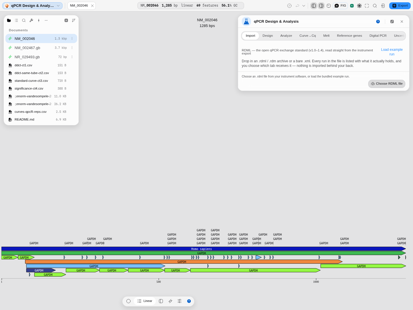
Every destination is a button, and the one that cannot work is disabled with the reason underneath
— this file has no <partitions> element, so Digital PCR is greyed out rather than failing later.
2. Fit the curves
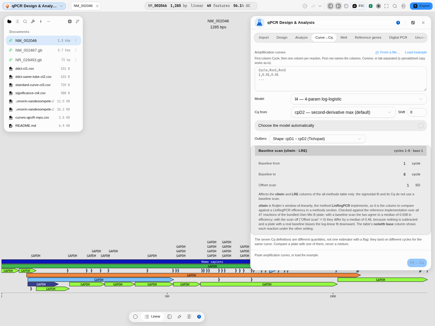
The curves arrive as text in the Curve→Cq tab. Tick Choose the model automatically — with eight
models available, letting a nested F-test or AICc pick is better than defaulting to l4 out of
habit — and press Fit → Cq.
Reaction C11 selected: Cq 25.27, cpD1 27.18, efficiency 57.7 %, R² 1.0000. Click any row to
plot that reaction.
3. Read what the fit is telling you — before you read the Cq
This is the step most workflows skip, and it is the one that decides whether the numbers mean anything.
✕marks a fit that describes no amplification. On this run, 14 of the 47 reactions — the 1 and 1 dilutions, which were inhibited, plus two wells whose fit failed outright. Their Cq is what the definition returns on that curve, not a measurement of a product. Exclude them.⚠is a different question: this reaction behaves unlike the rest of its group. A well can carry either mark, both, or neither.- The warning above the table names reactions, not conditions. Here it says the baseline crosses
zero in
I13andK11, so the ratio-based Cq definitions divide across a sign change and their efficiency is not a real number. It names the wells, the estimator affected and the fix.
4. Check the efficiency four independent ways
Load the tab's own four-reaction example (Load example) for a clean pair of replicates, and look at the efficiency table underneath the fit.
The four columns are four different algorithms — the sigmoidal fit, a sliding log-linear window, an exponential-phase fit and LRE — run on the same curve. Agreement between them is the evidence a well is clean. Disagreement is not a bug in one of them; it means the curve does not have a well-defined exponential phase, and any single efficiency you quote from it is a choice rather than a measurement.
| Reaction | sigfit | sliwin | window | expfit | LRE |
|---|---|---|---|---|---|
| F1.1 | 1.963 | 1.739 | 11–16 | 1.746 | 1.880 |
| F1.2 | 2.035 | 1.738 | 11–16 | 1.751 | 1.823 |
| F5.1 | 1.833 | 1.746 | 24–29 | 1.803 | 1.921 |
| F5.2 | 1.875 | 1.744 | 24–29 | 1.808 | 1.936 |
5. Put an interval on the Cq
Open Error bars on this Cq, keep the residual bootstrap, and press Resample. The fitted curve is resampled and refitted 200 times, and every readout comes back with the spread the observations actually support.
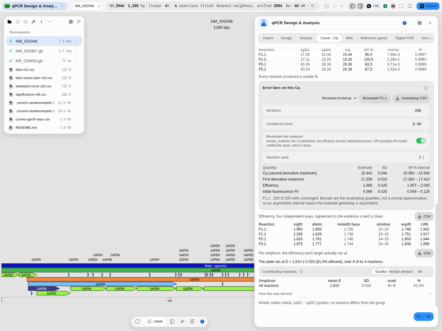
The same frame carries the four-reaction table, the "every reaction produced a usable fit" line and the four-way efficiency check — the whole tab in one state.
| Quantity | Estimate | SD | 95 % interval |
|---|---|---|---|
| Cq (second-derivative maximum) | 15.441 | 0.044 | 15.360 – 15.520 |
| First-derivative maximum | 17.359 | 0.023 | 17.310 – 17.400 |
| Efficiency | 1.965 | 0.025 | 1.917 – 2.018 |
| Initial fluorescence F0 | 0.066 | 0.025 | 0.021 – 0.113 |
Read the converged count. 200 of 200 means every resample refitted; a curve that only fits half
the time says so, instead of handing back a confident-looking interval built on the half that worked.
The bounds are resampling quantiles rather than a normal approximation, so an asymmetric interval
means the estimate genuinely is asymmetric.
Worked example
Open the qPCR & digital PCR starter, go to Curve→Cq, press Load example — a real
four-reaction run with two replicate pairs — then Fit → Cq with the defaults (l4, cpD2).
| Reaction | cpD1 | cpD2 | Cq | Efficiency | Residual variance | R² |
|---|---|---|---|---|---|---|
| F1.1 | 17.36 | 15.44 | 15.44 | 96.3% | 7.66e-3 | 0.9997 |
| F1.2 | 17.11 | 15.33 | 15.33 | 103.5% | 2.29e-2 | 0.9992 |
| F5.1 | 30.39 | 28.39 | 28.39 | 83.3% | 3.71e-3 | 0.9999 |
| F5.2 | 30.19 | 28.28 | 28.28 | 87.5% | 1.92e-3 | 0.9999 |
The replicate pairs agree to about a tenth of a cycle, which is what a clean replicate looks like. The efficiencies agree far less well — 96.3% against 103.5% for the same template — and that spread, not the Cq spread, is the thing to look at before trusting a quantification built on them.
The fit report for F1.1:
l4 coefficients   -12.0739, 0.0679, 11.3261, 17.5988     E ≈ 1.963
R² (qpcR) 0.9997   R² (textbook) 0.9997   RMSE 8.38e-2
AICc -92.95        BIC -84.40             Take-off 10.00   Midpoint 13.72
The run also raises a warning, and it is the most useful thing on the screen:
Baseline crosses zero in F1.1, F1.2, F5.1, F5.2. The spline estimators (Cq from maxRatio) divide consecutive readings, so a sign change puts a pole in the series and the efficiency there is not a real number. Use a model-based Cq on these reactions, raise the maxRatio baseline shift above the lowest reading (qpcR's own remedy), or re-export without baseline subtraction.
These curves were exported with the instrument's baseline subtraction already applied, so their early readings sit either side of zero. Every model-based definition is untroubled by that; the ratio-based one is not, because dividing consecutive readings across a sign change is division by something near zero. The panel names the reactions, the estimator and the fix, instead of returning a number that would look like a Cq.
Controls
Model — eight, in two families. The l family fits on the log scale, the b family on the raw
scale; within a family, parameters buy shape.
| Model | What the extra parameters buy |
|---|---|
l4 / b4 | The plain sigmoid: lower and upper asymptote, slope, inflection |
l5 / b5 | Asymmetry — the curve may rise and level at different rates |
l6 / b6 | A linear baseline drift |
l7 / b7 | A quadratic baseline |
l4 is the default and suits most clean runs. Reach for the six- and seven-parameter forms when the
early cycles slope instead of sitting flat: fitting drift explicitly is better than subtracting it by
eye.
Choose the model automatically. Fits the family and selects by information criterion rather than by your choice. Useful across a plate of mixed-quality wells — switch it off when you need every well analysed by the same model, which is what comparability requires.
Cq from — seven definitions.
| Definition | What it is |
|---|---|
| cpD2 | The second-derivative maximum, where the curve's acceleration peaks. The default, and what most instrument software reports |
| cpD1 | The first-derivative maximum — the steepest point. Always later than cpD2 |
| maxE | The cycle of maximum efficiency |
| expR | A point in the exponential region, derived from cpD2 and the efficiency there |
| Cy0 | Where a tangent taken at the first-derivative maximum crosses the x axis — built to stay robust when amplification is slightly inhibited |
| CQ | The cycle at 20% of the fluorescence at Cq |
| maxRatio | Model-free: a spline through the raw readings, then the maximum cycle-to-cycle ratio |
Shift. Offsets the cycle axis, for exports whose first row is not cycle 1.
Threshold. A fluorescence level on the plate's own scale. Set, every Cq is the cycle where the fitted curve crosses it, the classic threshold cycle, and it overrides Cq from. A reaction that never reaches the threshold reports no Cq and names the range it did reach. Blank, the Cq is read under Cq from. No value is offered as a default, because a threshold means nothing off its plate.
Baseline shift. Shown only under maxRatio. The ratio method divides consecutive readings, so a baseline near or across zero makes it explode; adding a constant to every reading first (qpcR's example uses 0.2) lifts the series clear of zero. It touches no other definition.
Smooth before the spline. Also maxRatio only: smooths the raw readings before the spline is drawn, which steadies the ratio on a noisy curve.
Amounts. The known template amount of each reaction, in the plate's column order, separated by
commas or spaces, with - for a reaction that has none. Each reaction given an amount reports its
calibration factor next to its initial fluorescence.
Fluorescence axis. Draws the plate's curves on the fluorescence as recorded or on its log10, where the exponential phase is a straight line and a threshold set in it reads as one horizontal rule. Readings at or below zero cannot be drawn on a log axis; they are left out and counted.
Outliers — two tests asking different questions. Shape compares the gap between a well's own cpD1 and cpD2 against its group, so a reaction whose curve is a different shape from its replicates is flagged even when its Cq looks reasonable. Efficiency Z-score tests the per-reaction efficiency against the group instead. A well can pass one and fail the other, and which it fails tells you what went wrong.
Baseline scan — from cycle, to cycle, offset scan SD. Sets the cycles treated as baseline. The panel states its own scope, and it is worth repeating: this affects the two baseline-dependent columns of the all-methods table only. The sigmoidal fit and its Cq do not use a baseline scan at all, because the model fits the baseline as parameters instead of subtracting it first.
Choosing the model by reduced chi-square
Alongside the two nested tests and AICc weights there is a fourth criterion: reduced chi-square, which asks a different question from all three. The others compare models against each other; this one compares a model against the measurement error your own plate exhibits. A value near 1 means the fit is as good as the data's own noise allows — larger means the model is missing structure, much smaller means it is fitting noise.
It needs an error per cycle, and the only honest source of one is repeated reactions. Name your
replicates the way every instrument export already does — F1.1, F1.2 — and the spread across them at
each cycle becomes that error; the panel prints where it came from ("4 replicates in 2 groups"). On a
plate with no replicates the criterion refuses before running rather than ranking models on a blank
number.
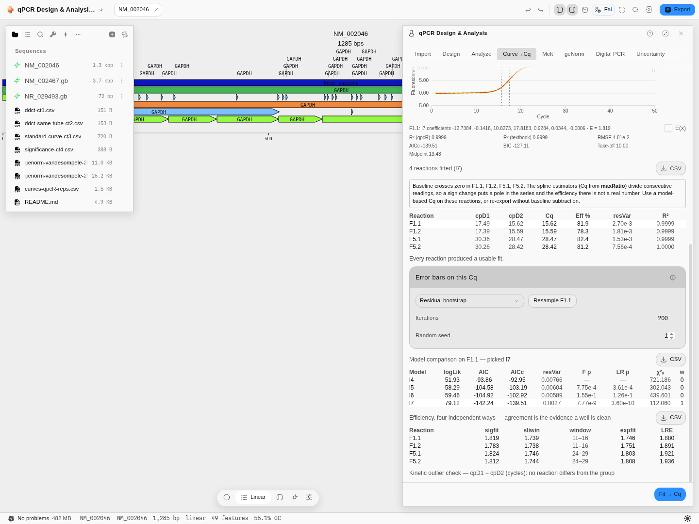
The shipped four-reaction example: χ²ᵥ reads 721 for l4, 302 for l5, 440 for l6 and 112 for l7. Ranked by distance from 1 that selects l7 — the same model AICc weights selects by an entirely different route, which is the useful part. All four values are far above 1, which says honestly that even the best of these models leaves structure behind relative to how tightly the replicates agree.
Algorithms you can choose
Every method above is a published one, labelled on the panel with the name it was published under. The efficiency table computes efficiency several independent ways for the same reaction — from the sigmoidal fit, from a window of linearity on the raw data, from an exponential fit to that window, and from a linear-regression-of-efficiency treatment — because agreement between methods that share no assumptions is the strongest available evidence that a well is clean.
| Method | Published as |
|---|---|
| Window-of-linearity efficiency, and the shape-based outlier test | Tichopad A, Dilger M, Schwarz G & Pfaffl MW, Nucleic Acids Research (2003) 31: e122 |
| Efficiency Z-score outlier test | Bar et al. (2003) |
| Cy0 | Guescini M, Sisti D, Rocchi MB, Stocchi L & Stocchi V, BMC Bioinformatics (2008) 9: 326 |
| maxRatio | Shain EB & Clemens JM, Nucleic Acids Research (2008) 36: e91 |
| Baseline-and-bias efficiency, the LinRegPCR treatment | Ruijter JM, Ramakers C, Hoogaars WM, Karlen Y, Bakker O, van den Hoff MJ & Moorman AF, Nucleic Acids Res (2009) 37: e45 |
| Linear regression of efficiency (LRE) | Rutledge RG & Stewart D, BMC Biotech (2008) 8: 47 |
The science
A PCR reaction is exponential only while primers and nucleotides are in excess. By the time fluorescence rises above the noise the reaction is already leaving that phase, so the exponential you want to characterise is one you can never observe directly. Every method here extrapolates back into it, and they differ in what they assume about the part you cannot see.
Fitting a sigmoid is one such assumption: that baseline, exponential and plateau are together described by a single smooth function whose parameters can be estimated — after which the derivatives are analytic rather than differences between noisy readings. cpD2 is then a property of the fitted function rather than of the individual points, which is what makes it stable enough to compare across a plate.
The ratio-based methods make the opposite trade. No model, so nothing to misfit; but every quantity is a ratio of adjacent readings, and therefore exposed to noise and — as the worked example shows — to a baseline that crosses zero.
Where the numbers come from. The models, the seven Cq definitions, the efficiency methods and both outlier tests are those implemented in the qpcR package for R, and the results here are checked against it directly: the same curves through both, compared value by value, re-runnable at any time. Where the two disagree, qpcR is treated as correct until proven otherwise.
How precise is that Cq?
A quantification cycle comes with no error bar from any instrument, and that is a real gap: two samples whose Cq differs by 0.3 may or may not be different, and nothing on the screen tells you which. Because the Cq is read off a fitted model rather than measured directly, its uncertainty is a property of how tightly your observations pin that model — so the way to measure it is to disturb the data and refit.
Two schemes, answering different questions:
- Residual bootstrap keeps the fitted curve, shuffles its residuals with replacement, adds them back and refits. It asks: how much would this Cq move if the noise had fallen differently?
- Jackknife leaves observations out and refits. It asks: does this fit rest on any one reading? — the question that catches a curve held up by a single point. How many it leaves out is yours to set: one is the classic delete-one jackknife, and leaving out more makes the answer less sensitive to any single influential cycle.
On reaction F1.1 of the bundled example, 200 bootstrap refits give a Cq of 15.441 with a 95 % interval of 15.360 – 15.520, an efficiency of 1.965 [1.917, 2.018], and an initial fluorescence of 0.066 [0.021, 0.113]. The interval on F0 is wide relative to its value, and that is the honest reading: the baseline is the least well determined part of a sigmoid fit.
The bounds are the resampling quantiles rather than a normal approximation, so an asymmetric interval means the estimate genuinely is asymmetric. The panel also reports how many refits converged — a curve that only fits half the time says so, instead of returning a confident interval built on the half that worked.
The confidence level is a control, and the readout names the level it used. 95 % is the usual choice and not a fixed one; ask for 99 % and the table says 99 %. A bound quoted without its level is not a bound anyone can compare with another.
You can also resample the coefficients alone. The readouts — the Cq under each definition, the efficiency, the initial fluorescence — are what the section is for and are on by default, but a run that only needs the model's own parameters is cheaper without them, and the panel says which it did.
Run it on the reaction you have plotted, not on the plate: each iteration is a full refit of a nonlinear model, so a few hundred of them is the cost of one reaction's error bar.
Limitations
- A Cq is not a quantity. Nothing on this tab knows your assay's standard curve or reference gene, so nothing here should be read as a fold change.
- A model can fit beautifully and still be the wrong model. R² near 0.9999 across all four example reactions does not make the four-parameter form right for them — only that it describes them well. Where you expect baseline drift, fit it rather than out-fitting it.
- maxRatio is unusable on baseline-subtracted exports whose readings cross zero, as the worked example shows. The panel detects the case and names it rather than silently falling back to another estimator, which would change the quantity without telling you.
- Efficiency disagreement between methods is diagnostic, not decorative — but the panel does not decide the well for you. What a 96.3% against 103.5% spread on two replicates means depends on your assay.
- The example run is four reactions. Real plates are 96 or 384 wells, and fitting cost is per reaction.
Compared with other tools
The short version: instrument software gives you a Cq. This tab gives you the Cq, the assumptions behind it, and a way to check every one of them.
Eight models, and a test that chooses between them. Four log-logistic shapes and four Baranyi shapes, with automatic selection by nested F-test, Akaike weights, residual-variance ratio or χ². A package that fits one curve shape and never names it is making a modelling decision on your behalf and not telling you which one.
Seven Cq definitions, computed together. cpD2 is the default because it is what most instruments approximate, but cpD1, maxE, expR, Cy0, CQ and maxRatio come off the same fit and sit beside it. If your Cq moves by a cycle when you change definition, that is a fact about your curve you should know before you publish it — not something buried in a vendor's algorithm.
Four independent efficiency estimators per reaction. Most tools report one efficiency, usually from a dilution series covering the whole plate. Here every well gets four, from four different algorithms, and their agreement is a per-well quality signal you can act on.
A confidence interval on the Cq itself. Almost nothing reports this, because it needs the curve resampled and refitted a few hundred times rather than a formula. You also get the converged fraction, so a badly-behaved curve is visible rather than smoothed over.
Fit quality shown, not hidden. Two R² definitions side by side (qpcR's own and the textbook one, because they differ and comparing against only the first is uncheckable), RMSE, AICc, BIC, residual variance, the take-off cycle and the midpoint — per reaction, next to the number they qualify.
Failures are named. A well whose fit describes no amplification is marked and listed; a baseline that crosses zero names the affected reactions and the estimator it breaks. Nothing here returns a plausible number in place of an honest refusal.
Checked against the reference implementation. Every estimator on this tab is validated against the published R package that defines it, over the whole of its own test corpus rather than a sample.
What it does not do: drive an instrument, read proprietary run files with no published schema, or turn a Cq into a copy number on its own — that needs a standard curve or a reference gene, next door.
Export
The per-reaction table and the all-methods efficiency table each export as CSV. What leaves this panel is numbers — the fitted curves are read here rather than exported as a figure.
API
The fitting, the seven Cq definitions, the efficiency methods and both outlier tests are reachable from the Python and R consoles inside the app, so a plate can be analysed in a loop rather than reaction by reaction.
Automation
The fit step is available as a workflow node — call_cq — so a run can be fitted and passed
onward without opening the tab, which is worth wiring when the same plate layout arrives every week.
It takes the same amplification table this tab takes and opens on the same model and the same Cq
definition, and it returns each reaction's efficiency and fit quality beside its Cq, so a step
downstream can act on a bad fit rather than inheriting it silently. Reactions that could not be
fitted are counted and named rather than dropped.
Every control this tab has, the node has. Which sigmoid is fitted, or letting the plate choose its own model and which criterion ranks them; which of the seven Cq definitions is reported and the cycle shift on it; which kinetic-outlier test judges the reaction shapes; and the cycle window the baseline scan runs over, with its offset. A run that could be tuned here and not there would be two different analyses under one name.
It returns what this tab shows rather than a Cq column alone: the model ranking when the plate chose its own, the four-estimator comparison with each failure named, the outlier verdicts — including the reactions the test could not measure, which come back as not judged with the reason rather than as passing — and the reactions whose baseline crosses zero, where a spline efficiency would otherwise report a confident but meaningless number.
(This page said the fit step was available as a node before one existed. It is accurate from 2026-09-03; the sentence is kept, corrected, rather than quietly rewritten.)
Provenance
A fit records the model, the Cq definition, the baseline window and the outlier test alongside its results, so a number that reaches a figure can be traced back to the assumptions that produced it. When citing, name the method from the table above and state which Cq definition you used — that one line is what makes a Cq comparable between two papers.
Related
Feeds it: your instrument's raw export. Follows it: qPCR Design & Analysis for ΔΔCt, standard curves and reference-gene stability; Digital PCR when the question is absolute rather than relative. An alternative to: the Cq your instrument software already reported — this tab exists so you can check that number instead of inheriting it. Melt Curves → Tm analyses the other half of the same run.