
Melting Temperature
Compute the melting temperature of an oligo under conditions you state, rather than under conditions a tool assumed.
| Reached by | Tools → Melting Temperature |
| Sample project | Primer test |
What it does
A melting temperature is not a property of a sequence. It is a property of a sequence in a buffer, at a concentration, under a model. Change any of those and the number changes, often by more than the margin you were designing against.
Most tools hide that. They pick a model, assume a buffer, and print one number. This panel makes all three explicit: you choose the thermodynamic model, state the actual buffer and strand concentrations, add the additives you are really using, and see what each one contributes.
How much it matters, on one real 20-mer, computed by this engine:
| Model, conditions | Tm |
|---|---|
| Breslauer 1986, Taq mix | 71.17 °C |
| NEB | 65.43 °C |
| Sugimoto 1996, Taq mix | 64.47 °C |
| SantaLucia & Hicks 2004, Taq mix | 61.48 °C |
| Allawi & SantaLucia 1997, Taq mix | 61.47 °C |
| Wallace rule | 60.00 °C |
| Allawi & SantaLucia 1997, Biopython defaults | 53.10 °C |
| GC formula, von Ahsen 2001 | 50.40 °C |
Same 20 bases. A 21 °C spread. Two of those rows differ only in buffer and strand concentration, and that alone is 8 °C. The panel exists so the number you carry to the bench is one you chose the assumptions for.
When you'd use this
Used in: Clone an insert into a vector, and prove it worked · Design primers, simulate the PCR, and predict the band
Three situations, and they are the reason this is a panel rather than a readout:
- You are designing primers and need the two of them to anneal at the same temperature. Reach for it from Primer Designer — which searches under exactly the conditions set here — and from PCR Simulation when the product is right but the reaction is not. Set the buffer to the mix you will actually pipette first; a pair matched under the wrong assumptions is matched at the wrong temperature.
- A calculated annealing temperature did not match the bench. This is the diagnostic use, and the answer is usually in the breakdown rather than the total: an additive nobody accounted for, a salt correction the other tool pinned, or a model from a different decade. DMSO is the one that hides best, because both tools may be applying a depression and simply not the same one — 5 % costs 3.75 °C under von Ahsen and 2.50 °C under Cullen & Bick, and neither is wrong. The table above is a 21 °C spread on twenty bases — the discrepancy you are chasing is often not an error at all.
- You are comparing against a number another tool gave you. Choose that tool's model and buffer explicitly and the two should meet. If they do not, one of you is applying a correction the other is not, and the per-correction lines say which.
The reach is wider than the panel, which is the thing to internalise: these conditions are the
application's conditions. The same TmFunc feeds the sequence inspector, Primer Designer's
search, Site-Directed Mutagenesis,
qPCR assay design, PCR and
Multiplex, and the primer design inside
Gibson, Golden Gate and
CRISPR. Changing the buffer here changes every Tm in the editor — a feature
when you set it once at the start of a design, and a surprise if you expect a scratchpad.
Each of those can be detached with an explicit override when a design genuinely runs in a different buffer, and the panel says which are detached. What none of them do any more is quietly disagree: before this was shared, a target Tm of 58 °C in a Gibson primer meant 58 °C in a buffer you never chose, and a guide's validation primers were designed in yet another.
Reach for something else when: you want a measured melt rather than a predicted one — that is Amplification Curves → Cq. If you want the whole molecule rather than one oligo, stay here: the melting map colours each base at a temperature you choose, and the melt curve plots the whole molecule melting across a temperature range. Both are described below.
Worked end to end: Clone an insert into a vector, and prove it worked.
What this computes
A melting temperature and everything it depends on, because the number is a property of a sequence in a buffer, at a concentration, under a model — and this panel makes all three explicit rather than picking for you.
- Tm under any of eight models — SantaLucia & Hicks 2004 (the default,
DNA_NN4), Allawi & SantaLucia 1997 (DNA_NN3), Sugimoto 1996 (DNA_NN2), Breslauer 1986 (DNA_NN1, which runs hot), pydna'stmbreslucfor dsDNA-binding-domain polymerases, the GC formula with eight published value sets, the Wallace rule (valid only under ~14 bases, and said so), and the NEB model. They disagree by up to 21 °C on the same twenty bases, which is the reason the choice is on screen - A second, independent axis: the salt correction, eight methods, Biopython's 0–7 named rather than numbered. Two rows of that comparison differ only in buffer and salt method, and that alone is 8 °C
- ΔH, ΔS and ΔG from the same table as the Tm, so a reading never mixes two models
- What each condition contributes — Na⁺, K⁺, Tris, Mg²⁺, dNTPs, DMSO, formamide, and the strand concentrations — as a term you can see rather than a correction folded into one number. Mg²⁺ is corrected for dNTP chelation, so raising dNTPs above Mg²⁺ removes the divalent contribution
- A third axis nobody expects to be a choice: how much DMSO costs you. Four depressions have been published and they do not agree — von Ahsen et al. 2001 at 0.75 °C per percent, Escara & Hutton 1980 at 0.675, Musielski et al. 1981 at 0.6, and Cullen & Bick 1976 at 0.5. On the 5 % DMSO a GC-rich template routinely needs, that is a 1.25 °C spread — larger than the difference many people would accept between two tools. All four are offered, checked against the same reference implementation (MELTING 5) that publishes them, and the breakdown names the one in force beside the degrees it removed, so a disagreement with another calculator can be traced to the coefficient rather than argued about. Type a coefficient of your own and the line says so instead of citing a paper that did not publish it
- Formamide under either published model — the linear rule of McConaughy et al. 1969 in percent by volume, or Blake & Delcourt 1996, which is molar and depends on the oligo's own GC fraction, so two primers in the same tube are depressed by different amounts
- Locked nucleic acid (LNA), when the probe you ordered has some. Write it as it is written on
the tube — an
Lafter each locked base,GTCGLAACAGC— and the melting temperature carries the per-neighbour increments McTigue, Peterson & Kahn (2004) measured over a hundred duplexes. A locked base sits in two nearest neighbours and both are charged, which is why one substitution moves a probe by degrees rather than by tenths, and the derivation names the two neighbours that paid it. A terminal locked base is refused rather than estimated: the paper measured none, and a number for a duplex nobody measured is worse than no number. Locked bases are only meaningful under a nearest-neighbour model, so the GC formula, the Wallace rule and the NEB model say so instead of quietly scoring the probe as plain DNA - The comparison itself: every model computed at once on the same oligo, under the same buffer, which is what turns "which model?" from an opinion into a measurement you can read
Why the default is SantaLucia & Hicks 2004 with the Taq mix preset — agreement, not authority. It is what pydna computes with, and pydna is what this workbench's cloning engines are checked against byte for byte. Choosing it means the Tm you read here is the one the rest of the app is reasoning with; the primer designer, the PCR simulation and the mutagenesis panels all pull the same conditions.
What it does not compute: whether your reaction will work. A Tm is a duplex property, not a prediction about a polymerase, an enzyme lot, or a thermocycler's block calibration.
Where it lives
Tools → Melting Temperature opens it in the right rail. Right-click on the canvas → Melting temperature opens it seeded from the current selection, so a primer you have highlighted arrives already loaded.
Its reach goes further than the panel:
- These conditions are the app's conditions. The same
TmFuncthis panel builds is what the sequence inspector readout, the Primer Designer's search, Mutagenesis, qPCR, PCR, Multiplex and the primer design inside Gibson, Golden Gate and CRISPR compute with — nine surfaces. Change the buffer here and every Tm in the editor follows. Individual tools may hold an override, and the Editing selector at the top of the Conditions tab says which, but there is one shared default rather than nine hard-coded ones. - The model choice travels with the buffer. Picking Breslauer 1986 here means Breslauer 1986 in the Primer Designer and in the PCR product readouts, not just in this panel's headline number. The four nearest-neighbour tables are up to 7.5 °C apart on a single 20-mer, so a model that applied to one surface and not the next would be worse than no choice at all.
- The melting map is the panel's other half. Drag a temperature and the plasmid recolours by predicted helicity, so a region that opens early is visible on the map rather than inferred from a table.
- The melt curve is the same physics read the other way round: instead of one temperature across every base, it is every temperature across the whole molecule. The two share a single temperature, so clicking a point on the curve recolours the map, and moving the map's slider moves the curve's marker. You can leave the map painted and work from the curve.
Inputs and outputs
In: a sequence, from the canvas selection, the open record, or typed. Plus the conditions: model, buffer, strand concentrations, additives.
Out: the melting temperature, the corrections applied to reach it broken out one by one, and for nearest-neighbour models the underlying ΔH, ΔS and ΔG. The melting map outputs a helicity band per region at the chosen temperature; the melt curve outputs helicity and its rate of change across a temperature range, a Tm50, and the melting domains it resolves — exportable as CSV.
What it will not do:
- Fields a model does not use are disabled, not ignored. The Wallace rule reads nothing but base counts, so its buffer fields go dead and say why. The GC formulas read the buffer but pin their own salt-correction method, so that one dropdown is disabled with the reason next to it. A knob that silently does nothing is worse than an absent one.
- Betaine and glycerol are not offered. See Limitations.
Demo
Not recorded yet. The obvious screencast is the melting map: drag the temperature slider and watch the plasmid recolour. Two still frames of that exact flow are under Screenshots in the meantime.
Worked example
The primer below is the M13 forward priming region, a universal sequencing primer, 20 bases with 10 G or C, so 50% GC by eye:
GTAAAACGACGGCCAGTGAAUnder the Taq mix (pydna default) preset, which is DNA_NN4, 250 nM each strand, 40 mM Na, 75 mM Tris, 1.5 mM Mg, 0.8 mM dNTP, Owczarzy 2008 salt correction:
Tm      61.48 °C
dH    -157.0 kcal/mol
dS    -424.3 cal/(mol·K)
dG     -25.40 kcal/mol
Now add DMSO, which is what the additive breakdown is for:
| DMSO | Tm | Change |
|---|---|---|
| 0% | 61.48 °C | |
| 5% | 57.73 °C | -3.75 °C |
| 10% | 53.98 °C | -7.50 °C |
That is 0.75 °C per percent DMSO, applied linearly, and it is the single most common reason a calculated annealing temperature does not match the bench. The panel shows this as its own line rather than folding it into the total, so the correction is attributable.
0.75 is one of four published coefficients, and which one you pick is a real choice. The DMSO depression has been measured four times, on different systems, and the answers do not agree:
| Model | °C lost per % DMSO | 8% DMSO costs |
|---|---|---|
| von Ahsen and colleagues (2001) | 0.75 | 6.00 °C |
| Escara and Hutton (1980) | 0.675 | 5.40 °C |
| Musielski and colleagues (1981) | 0.6 | 4.80 °C |
| Cullen and Bick (1976) | 0.5 | 4.00 °C |
All four are offered, each named with its paper, and von Ahsen is the default because it is the one measured under PCR conditions. The spread between them at 8% DMSO is 2 °C, which is larger than most people's annealing-temperature safety margin, so a Tm quoted without saying which coefficient produced it is not reproducible. Whichever you choose is named beside the number it produced and in the derivation chain, and a coefficient of your own can be entered instead. The values are checked against MELTING 5, which is the reference implementation that carries all four.
Switching only the model, with the same buffer, gives the first table on this page. Switching only the conditions, from the Taq mix to Biopython's defaults (25 nM strands, 50 mM Na, no Mg, salt method 5), moves the same Allawi & SantaLucia number from 61.47 °C to 53.10 °C.
The melt curve
A long molecule does not have a melting temperature. It has several. The nearest-neighbour Tm at the top of this page answers a two-state question — an oligo is either annealed or it is not — and that question stops being the right one somewhere around a few dozen bases. A plasmid melts in pieces: an AT-rich stretch opens while a GC-rich one is still fully paired, and the molecule passes through a series of partly-open states that no single number describes.
The Melt curve tab plots that directly.
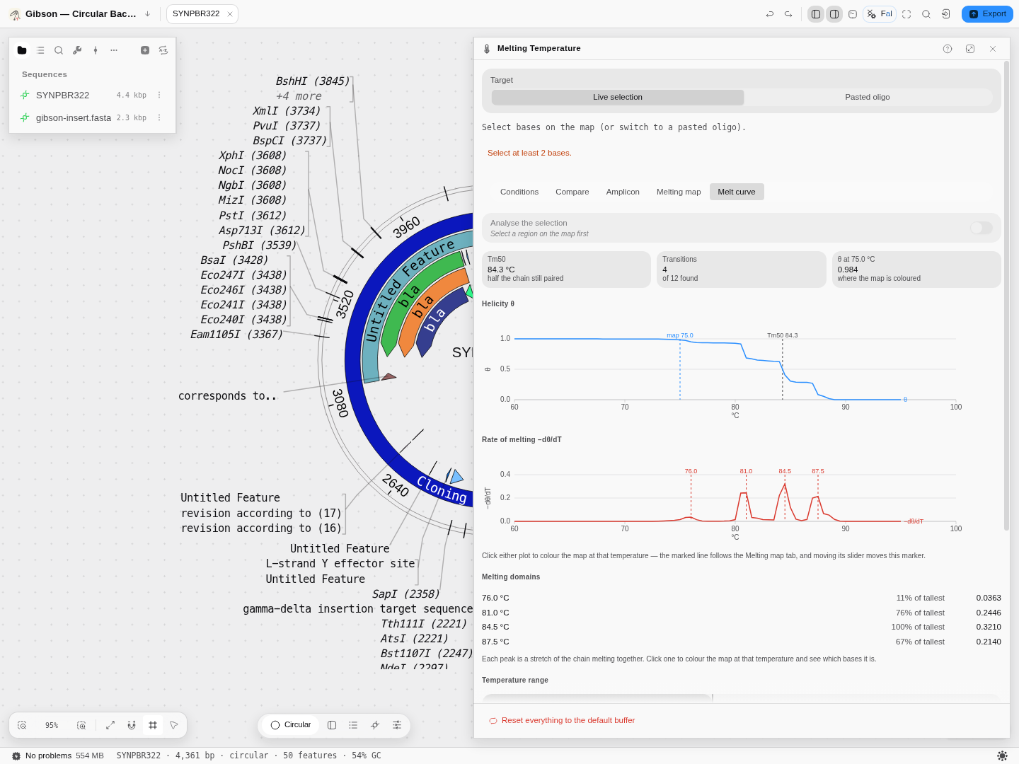
Real pBR322, 4,361 bp. The upper plot is helicity; the lower one is its rate of change. The four peaks are four separately-melting domains, and the staircase above them is the same four events seen as drops in the fraction still paired.
Reading the two plots
θ (theta), the upper plot, is the fraction of the molecule still base-paired at each temperature — 1.0 when the duplex is intact, 0 when it is fully separated. It is a probability averaged over every base, not a yes/no. Where it is flat, nothing is happening; where it drops, something is melting.
−dθ/dT, the lower plot, is how fast that is happening. Each peak marks a temperature at which a stretch of the molecule comes apart cooperatively — a melting domain. This is the same quantity a high-resolution-melt instrument records as a derivative peak, which is why the shape is familiar even though these values are predicted rather than measured.
Tm50 is marked on the upper plot: the temperature at which half the molecule is still paired. Treat it as a summary, not as a mechanism — on a multi-domain molecule it can fall between two real transitions and correspond to nothing that physically happens at that temperature. If the range you chose never reaches 50 %, the panel says so rather than reporting the edge of your own window as a melting temperature.
Melting domains
Each peak is listed underneath with its temperature and its height relative to the tallest. Click one and the map colours at that temperature, which is how you find out which bases the peak is: the domain that opens first is usually the one that matters, and on a plasmid it is often the AT-rich regulatory region rather than the coding sequence.
What the numbers rest on
The curve is a Poland–Scheraga partition function (the Tøstesen 2003 formulation) over SantaLucia-1998 nearest-neighbour parameters. In plain terms: rather than asking whether the duplex as a whole is open, it sums over every possible arrangement of helical and open stretches along the chain, weighting each by its energy. That is why it can show one region melting while another holds, and it is a genuinely different computation from sliding a two-state oligo Tm along a window — an approach that cannot represent cooperativity at all.
The implementation is checked byte-for-byte against DECIPHER's MeltDNA, the Bioconductor
reference for this calculation, across every output type it produces.
The salt comes from the Conditions tab, like everything else in this panel. Raising Na⁺ stabilises the duplex and moves the whole curve to higher temperatures; on the fragment used for the worked example, dropping from 0.2 M to 0.05 M moves Tm50 by about 8 °C.
Controls on this tab
- From, To and Step. The default 60–95 °C at 0.5 °C is the window and resolution an HRM instrument runs. Widen the range if the curve has not finished melting at the top — a molecule that is still 98 % paired at 95 °C has no Tm50, and the panel will tell you so rather than invent one. A finer step resolves close domains at a proportional cost in computation.
- Show the rate of melting. Turns the −dθ/dT plot on and off.
- Smallest peak listed. A display filter on the domain list and its markers, as a share of the tallest peak. It changes nothing that is computed — it only decides how much of the fine structure is worth showing you. Set it to 0 to see every local maximum.
- Analyze the selection. Restricts both the curve and the map to the selected region, which is how you ask about one insert rather than the whole vector.
- Export the curve as CSV — every grid temperature with its θ and −dθ/dT, and the domains flagged.
Limits
The model is validated up to 100,000 base pairs; past that the panel refuses rather than extrapolating, and asks you to select a region. Below three bases there is nothing to melt.
Controls
Model. Eight, each labelled with its source:
| Model | What it is |
|---|---|
| Allawi & SantaLucia 1997 | Nearest neighbour, DNA_NN3. The pydna and QUEEN default |
| SantaLucia & Hicks 2004 | Nearest neighbour, DNA_NN4. The unified table, pydna tm_default |
| Sugimoto 1996 | Nearest neighbour, DNA_NN2 |
| Breslauer 1986 | Nearest neighbour, DNA_NN1. The oldest table, and it runs hot |
pydna tmbresluc | Breslauer matrices for dsDNA-binding-domain polymerases (Phusion, Q5) |
| GC formula | Biopython Tm_GC, with eight published value sets to choose from |
| Wallace rule | 2 °C per A or T, 4 °C per G or C. Valid only under about 14 bases |
| NEB | The Teselagen NEB model |
Target. Live selection follows whatever is selected in the editor; Pasted oligo takes a sequence you type. The Amplicon tab treats the target as a PCR product: give it the Fwd and Rev primers (or use the primers annotated on this record) and it gives the annealing temperature for both polymerase families.
Conditions. One set of reaction conditions is shared by every tool that computes a melting temperature. Editing picks whose conditions you are changing, and Give it its own conditions detaches that tool from the shared set.
Buffer, all in mM:
| Control | Default (Taq mix) |
|---|---|
| Na⁺ | 40 |
| K⁺ | 0 |
| Tris | 75 |
| Mg²⁺ | 1.5 |
| dNTPs | 0.8 |
| Correction | Owczarzy 2008 (Mg²⁺) |
Correction is the salt-correction method, Biopython's 0 to 7 named rather than numbered: none · Schildkraut & Lifson 1965 · Wetmur 1991 · SantaLucia 1996 · SantaLucia 1998 (1) · SantaLucia 1998 (2) · Owczarzy 2004 · Owczarzy 2008 (Mg²⁺). dNTPs matter because they chelate magnesium, so the free Mg²⁺ the correction sees is lower than the Mg²⁺ you pipetted.
Strand concentration. Strand 1 and Strand 2 in nM (250 each by default), plus Self-comp., which halves the concentration term because a self-complementary oligo anneals to itself.
Value set. Shown for the GC formula only: which of the eight published parameter sets it uses.
Additives. DMSO percentage under the DMSO model you pick, one of the four published depression models (von Ahsen 2001 · Escara and Hutton 1980 · Musielski 1981 · Cullen and Bick 1976) or a coefficient of your own in DMSO factor (°C per percent, 0.75 by default), and formamide under the Formamide model, either the linear percent form or the GC-dependent molar one. The linear form's Formamide factor is 0.65 °C per percent by default; published values run 0.6–0.72. The additives apply wherever a melting temperature is computed, not only on this page: set DMSO here and the PCR, multiplex and primer-design temperatures move with it.
Presets, each quoted from its upstream source and pinned by a test:
| Preset | What it reproduces |
|---|---|
| Taq mix | pydna tm_default: DNA_NN4, 250 nM, 40 Na / 75 Tris / 1.5 Mg / 0.8 dNTP, salt method 7 |
| Phusion / Q5 | pydna tm_dbd: DNA_NN3, 250 nM, 50 Na / 1.5 Mg / 0.8 dNTP, salt method 1 |
| Biopython defaults | Bio.SeqUtils.MeltingTemp.Tm_NN: DNA_NN3, 25 nM, 50 mM Na, salt method 5 |
| QuickChange | Biopython Tm_GC value set "QuickChange", the Tm Mutation Maker selects on |
| NEB | calculateNebTm defaults: 50 mM monovalent, 500 nM primer |
Melting map. A temperature, and helicity bands painted onto the canvas. It reads the same buffer as everything else, so moving Na⁺ in the conditions moves the map. The painting survives while you move between tabs, so you can leave it on and drive the temperature from the melt curve.
Melt curve. Temperature range, step, the rate-of-melting plot and the peak filter — described in full under The melt curve.
The melting map, in full
The other tabs answer "at what temperature does this oligo come apart?". This one answers a different question — "at this temperature, which parts of my molecule are still double-stranded?" — and the answer is a value per base, not one number for the whole thing.
What is computed. For the temperature you set, the probability that each base is still paired, given every helix-and-coil configuration the chain can adopt. That is a partition function over the whole molecule, so a base's fate depends on its neighbours: an AT-rich stretch does not open in isolation, it opens with the domain around it, and a GC clamp on one side can hold it shut. This is why the picture is domains rather than a GC plot.
The controls, and what each one changes:
| Control | What it does |
|---|---|
| Paint melting on the sequence | Turns the overlay on. It is a highlight only — your record is never modified, and the bands clear when the panel closes |
| Temperature | The only parameter of the profile itself. Type it or drag it; the map recolours as you move, because changing it is a re-read of the same computation, not a new run |
| Analyze the selection | Restricts the profile to the highlighted region instead of the whole molecule. Useful when one insert is the question and the vector is noise |
| Buffer, in the Conditions tab | Salt enters the calculation as a monovalent-equivalent. One buffer for the whole application, so the map and the primer Tms cannot disagree |
What you read off it:
- Mean helicity — the fraction of bases still paired, averaged over the region. 1.0 is fully duplex, 0.0 fully melted.
- Melting domains — how many contiguous stretches share a helicity band. Domain boundaries are where the molecule comes apart, and they are what the ring makes visible.
- The five bands, in order: paired (≥0.9) · mostly paired (≥0.7) · opening (≥0.5) · mostly open (≥0.2) · open (≥0). Each band is one span on the map with its own colour and label.
Read it by scanning up in temperature. Set a temperature where most of the molecule is still paired, then raise it: the region that turns colour first is the one that opens first. That is the region that will breathe in a PCR, be accessible to a probe, or dominate a high-resolution melt.
The size limit is an authority limit, not a performance one. The map is offered up to 100,000 base pairs, because that is the range the underlying loop-entropy approximation is documented as valid over. Beyond it the panel refuses with the reason stated rather than drawing something it cannot defend.
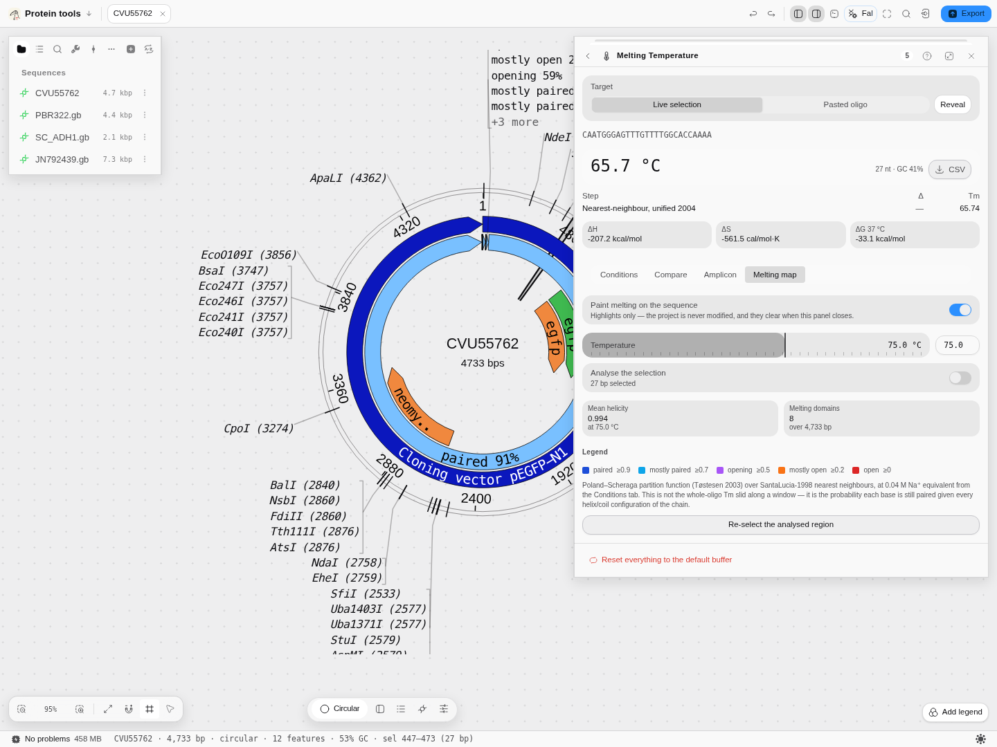
A 4,733 bp plasmid at 75.0 °C: mean helicity 0.994 across 8 melting domains, nearly all of it still paired, with the legend naming the five bands and the method line naming the model and the salt it used.
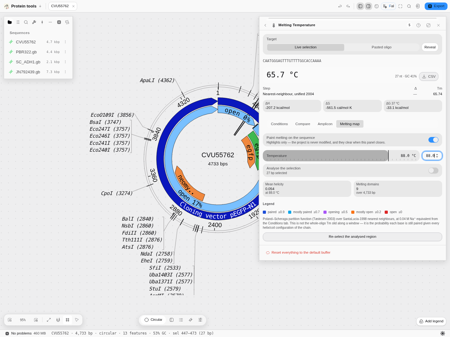
The same molecule at 88.0 °C — mean helicity 0.054 over 9 domains. The bands that read "paired 91%" now read "open 17%" and "open 0%". Nothing was re-run; only the temperature moved.
The Oligo tab — the spec sheet for the tube in your hand
A Tm tells you how an oligo behaves. It does not tell you how much of it you have, and that is the other question you open an oligo calculator for. The Oligo tab answers it for whatever is selected on the canvas or pasted above.
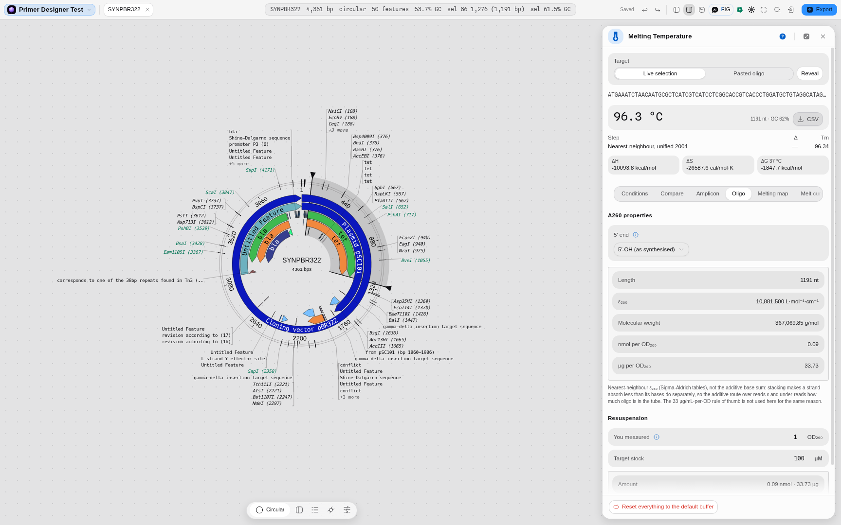
What it gives you
| Readout | What it is | What you do with it |
|---|---|---|
| ε₂₆₀ | Molar extinction coefficient at 260 nm, L·mol⁻¹·cm⁻¹ | Turns an absorbance into a concentration |
| Molecular weight | Average mass, g/mol | Turns moles into micrograms |
| nmol per OD₂₆₀ | How much oligo one absorbance unit represents | The number on a supplier's tube |
| µg per OD₂₆₀ | The same amount by mass | Cross-checks a nanodrop reading |
| Resuspension volume | µL of buffer for the stock you want | What you actually pipette |
Why not just add the bases up
Because stacking. Bases in a strand absorb less UV than the same bases would separately — hypochromicity — so summing the four single-base coefficients over-reads ε₂₆₀, and an over-read ε under-reads how much oligo is in your tube. You end up with a stock more concentrated than the label says, and every dilution from it inherits the error.
The tab uses the nearest-neighbour treatment instead: each overlapping dinucleotide contributes its own measured coefficient, and the interior bases — counted twice by two overlapping pairs — are subtracted once. The two terminal bases are counted once and are not subtracted, which is the step that is easy to get wrong and invisible afterwards.
For the same reason the tab does not use the "1 OD₂₆₀ = 33 µg/mL" rule of thumb. That constant is an average over base composition; for a real sequence it can be off by tens of percent. (On a long mixed-composition selection the nearest-neighbour answer does converge on roughly 33 µg/OD, which is where the rule comes from — it is the short, composition-skewed oligos you actually order where it fails.)
The 5′ end is a real choice, not a detail
Set 5′ end to match what you ordered:
- 5′-OH (as synthesised) — the default, and what a synthesiser ships unless you paid for phosphorylation.
- 5′-phosphate — kinased oligos, and strands considered as part of a cut molecule.
They differ by one HPO₃, 79.98 Da. On a 24-mer that is about 1 % of the mass, so it moves µg/OD₂₆₀ by 1 % and nothing else — small, but it is the difference between two right answers to two different questions, so the tab asks rather than assuming.
Resuspension
Enter the OD₂₆₀ you measured (or the amount the supplier states) and the stock concentration you
want, and the tab gives the volume. There is no fitted parameter in it: at a 1 cm path length one
absorbance unit is 1/ε mol/L, so the arithmetic follows from Beer–Lambert and the ε₂₆₀ above.
Where the numbers come from
The coefficients are the published Sigma-Aldrich single-base and dinucleotide tables, and every value this tab shows is checked against the reference implementation that ships them — over all four single bases, all sixteen dinucleotides, all sixty-four trinucleotides and a corpus of real primers, with the molecular weights independently cross-checked against Biopython.
Single strand or duplex — pick the molecule you actually have
Set Molecule to match what is in the tube. It is not a label; it changes every number below it.
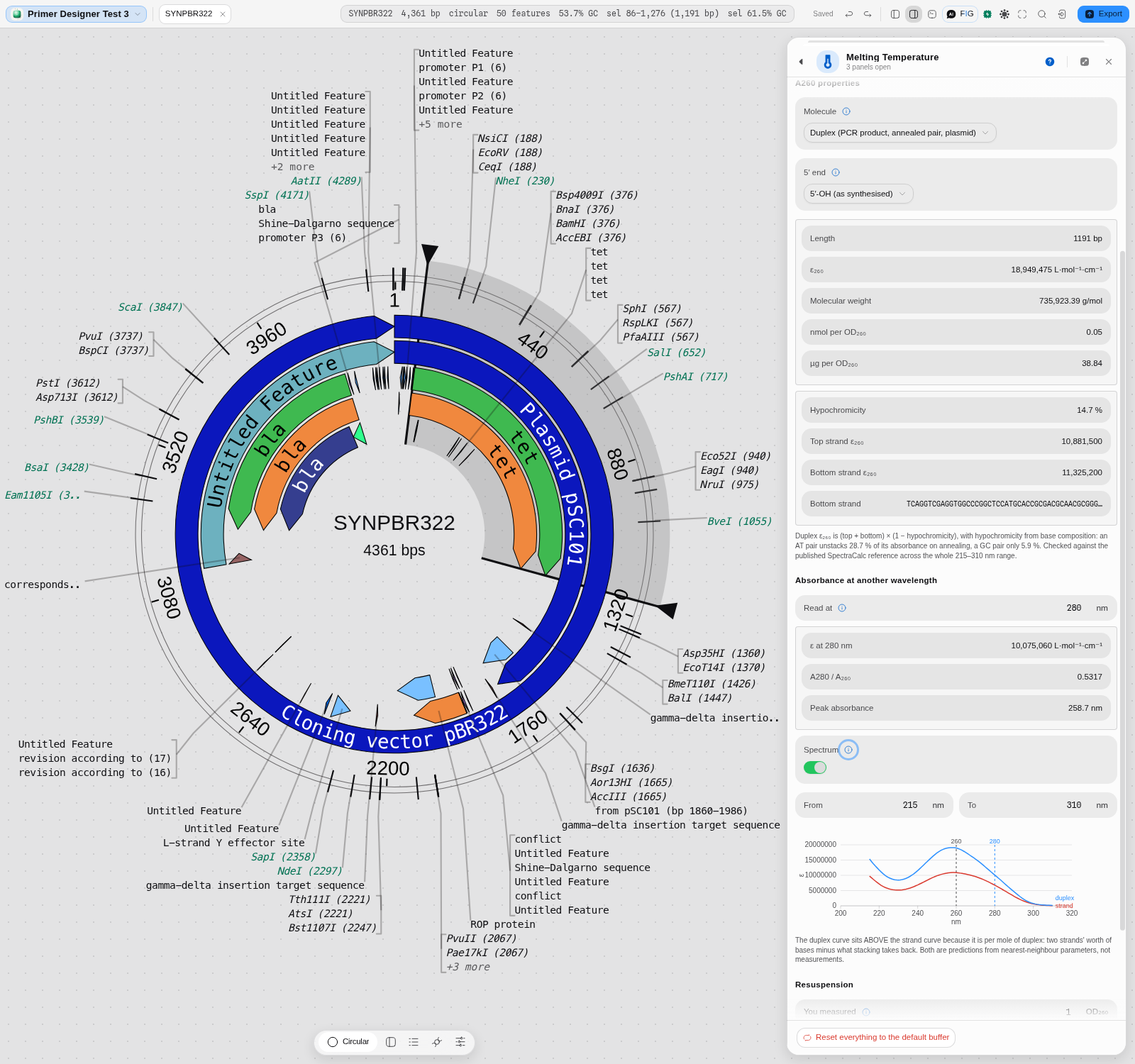
A duplex does not absorb what its two strands absorb apart. Stacking across the helix removes a chunk of the 260 nm signal, and how big a chunk depends on base composition: an AT pair loses 28.7 % of its absorbance on annealing, a GC pair only 5.9 %. So reading a PCR product, a plasmid or an annealed pair off the single-strand ε over-reads ε and under-reads how much DNA you have — the same direction as the additive-bases mistake above, and usually bigger.
Follow along on the tet gene of pBR322 (select it on the map, 1,191 bp):
- Molecule → Single strand. ε₂₆₀ reads 10,881,500.
- Molecule → Duplex. ε₂₆₀ becomes 18,949,475 — not 2 × the strand value, because the duplex row below shows the two strands at 10,881,500 and 11,325,200 and a hypochromicity of 14.7 % taken off their sum.
- µg per OD₂₆₀ moves from 33.73 to 38.84. That is the number that decides your dilution.
The duplex block also shows the bottom strand it built and both strand extinctions, so you can see where the answer came from rather than being handed one number.
Absorbance at any wavelength, and the whole spectrum
Under Read at, pick any wavelength from 215 to 310 nm and the tab gives ε at that wavelength
and the A(λ)/A₂₆₀ ratio. Set it to 280 and the tet duplex reads 0.5317 — the ~0.5 that a
spectrophotometer prints for clean DNA, which is why A260/A280 works as a purity check at all.
Turn Spectrum on for the whole predicted curve between From and To (nm), single strand and duplex together, with 260 nm and your chosen wavelength marked. The duplex curve sits above the strand curve because it is per mole of duplex: two strands' worth of bases, minus what stacking takes back.
A pitfall worth knowing: the Peak absorbance readout is a base-composition estimate of where the maximum falls (256–266 nm depending on your sequence), and it is not the argmax of the plotted curve. They can differ by a nanometre or two. Both are shown rather than one silently standing in for the other.
Labelled probes: dyes, quenchers and modified bases
Write a modification in brackets and the tab accounts for it:
[6-FAM]TCACTGGTGGCTCTTTTGCAGGTG[BHQ-1]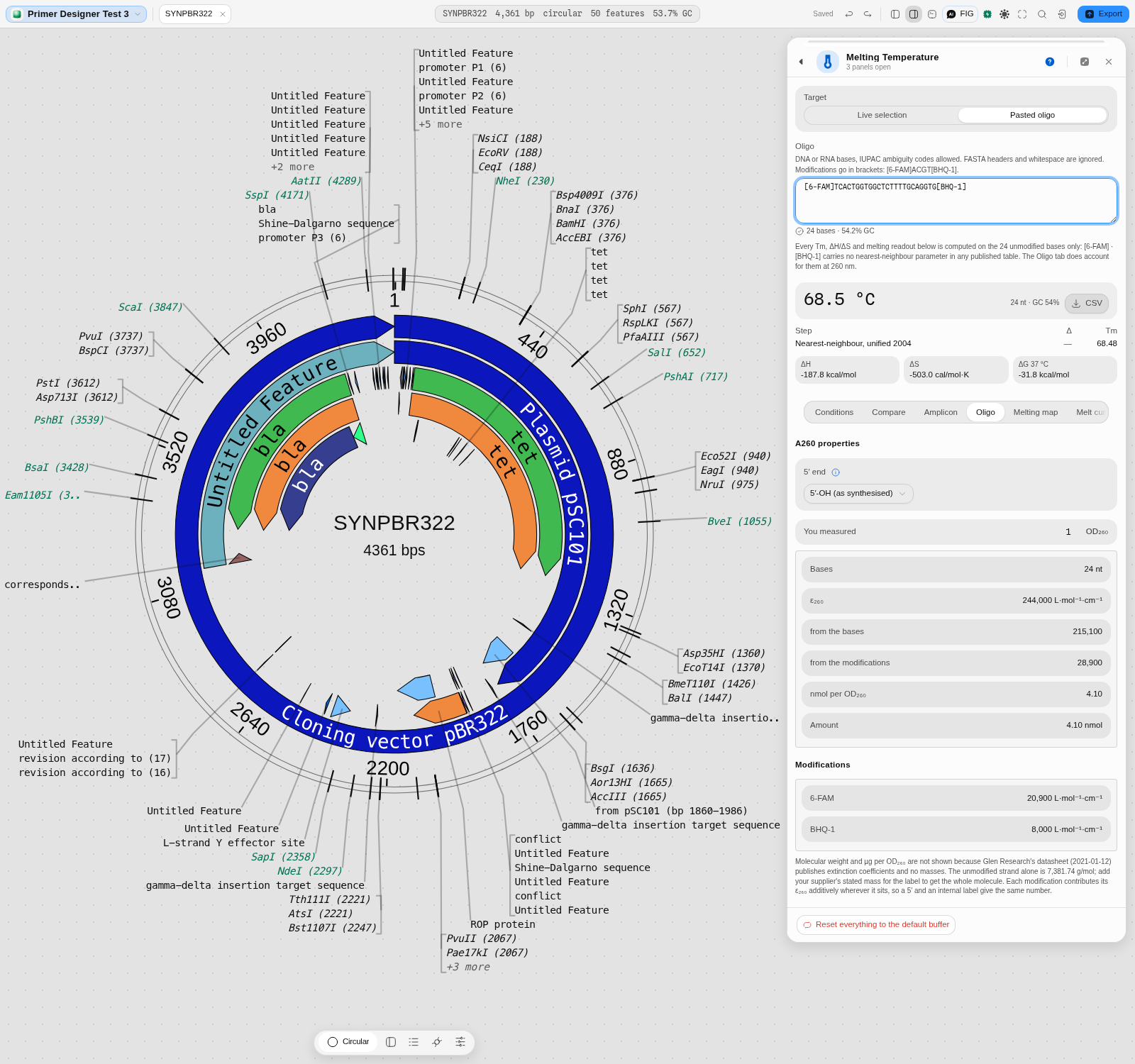
This is the case where guessing costs you most: a fluorophore alone can contribute more at 260 nm than several bases do. On the probe above, ε₂₆₀ is 244,000 — 215,100 from the 24 bases and 28,900 from the two labels (6-FAM 20,900, BHQ-1 8,000). Ignore the labels and you over-read the concentration of every probe you make up by about 12 %.
Around 75 modifications are recognised — modified nucleosides (7-deaza-dA, 5-Me-dC, inosine, 2-aminopurine, 5-nitroindole, LNA-adjacent analogues …), the common dyes (6-FAM, HEX, TET, TAMRA, Cy3, Cy3.5, Cy5, Cy5.5, Yakima Yellow, Redmond Red …) and the quenchers (BHQ-0/1/2/3, Dabcyl, Eclipse, MGB). Biotin and cholesterol are recognised as contributing nothing at 260 nm, which is a real answer rather than a missing one.
Three things the tab will refuse to guess, and each refusal names what to do:
-
A modification with no published coefficient. Some names in circulation have no value in any datasheet we can cite; those are absent rather than approximated, and the message says so.
-
A name the datasheet publishes twice with two different values.
Fluorescein-dTis one: 7,100 in the modified-nucleoside table and 38,800 in the fluorescence table — a 5.5× gap that would move your probe's concentration threefold. The tab shows both and asks which you mean.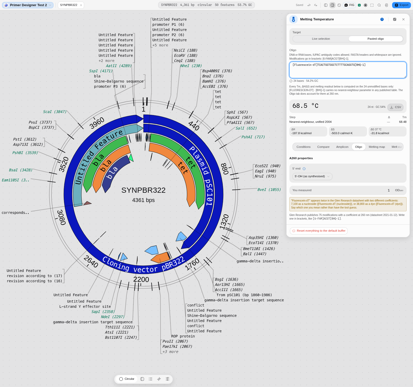
-
A mass. The datasheet publishes extinction coefficients and no masses, so molecular weight and µg/OD₂₆₀ are not shown for a labelled oligo. The unmodified strand's mass is given as exactly that; add your supplier's stated mass for the label to get the whole molecule. nmol/OD₂₆₀ needs only ε and is reported normally.
One limit of the model, and it is the standard one: a modification contributes its coefficient additively wherever it sits, so a 5′ label and an internal label of the same dye give the same number. That is what the vendors' own instructions say to do, not a shortcut taken here.
Limits
- Unmodified A, C, G and T outside the brackets. A degenerate base (N, R, Y …) is still refused with a reason rather than approximated.
- The duplex model assumes the two strands are fully complementary. It builds the reverse complement of what you gave it; a real mismatched or bulged duplex melts and absorbs differently.
Algorithms you can choose
This is the tool where the section matters most, because the choice is the product. Eight models ship, and they are not eight opinions about one number — they answer different questions, were measured by different groups under different conditions, and disagree by up to 21 °C on the same twenty bases. Nothing here picks a winner for you; the panel's job is to make the choice explicit and attributable.
| Model | The question it answers | Default for | Citation |
|---|---|---|---|
| SantaLucia & Hicks 2004 | "What does the unified nearest-neighbour table say?" — the modern consensus set, DNA_NN4 | pydna's tm_default, and the Taq mix preset | SantaLucia & Hicks, Annu Rev Biophys Biomol Struct 33 (2004) |
| Allawi & SantaLucia 1997 | The immediately preceding NN table, DNA_NN3 | pydna's tm_dbd, QUEEN, Biopython's Tm_NN | Allawi & SantaLucia, Biochemistry 36 (1997) |
| Sugimoto 1996 | An independently measured NN table, DNA_NN2 | — | Sugimoto et al., Nucleic Acids Res 24 (1996) |
| Breslauer 1986 | The original NN table, DNA_NN1. It runs hot — 71.17 °C where the 2004 table says 61.48 °C | — | Breslauer et al., PNAS 83 (1986) |
pydna tmbresluc | "What Tm does a dsDNA-binding-domain polymerase see?" Breslauer matrices, for Phusion and Q5 | the Phusion / Q5 preset | pydna, after Finnzymes' own calculator |
| GC formula | "What does the GC-content shortcut say?", with eight published value sets | the QuickChange preset, the set Mutation Maker selects on | Biopython Tm_GC; von Ahsen et al. 2001 among the value sets |
| Wallace rule | 2 °C per A/T, 4 °C per G/C. Valid only under ~14 bases | — | Wallace et al. (1979) |
| NEB | The Teselagen NEB model, matching NEB's own calculator | the NEB preset | Teselagen calculateNebTm |
The default is SantaLucia & Hicks 2004 with the Taq mix preset, and the reason is agreement, not authority: it is what pydna computes with, and pydna is what the cloning engines in this workbench are checked against, byte for byte. Choosing it means the Tm you read here is the Tm the rest of the app is reasoning with. Switch models and the number on screen moves immediately — the table at the top of this page is that experiment run once.
A second axis, and it is not a model choice: the salt-correction method, eight of them, Biopython's 0–7 named rather than numbered. Two rows of the opening table differ only in buffer and salt method and that alone is 8 °C. A model choice without a stated buffer is half an answer.
Bring your own. @ports/tm exposes each model directly, so the same functions the panel calls
are callable from the consoles or from your own code — see API. Every one is a
same implementation, so a number you get there is byte-identical to the panel's.
RNA and RNA/DNA hybrids
Tm models are measured on a particular chemistry, and the tables are not interchangeable. Four of the models here are not DNA/DNA:
| Model | Chemistry | Reach for it when |
|---|---|---|
| RNA/RNA, Xia 1998 | RNA duplex | The standard Watson–Crick RNA parameters. The default choice for an siRNA or an RNA duplex |
| RNA/RNA, Chen 2012 | RNA duplex, GU wobble | Your duplex contains GU pairs. The only table here that tabulates them, so a wobble is not scored as the mismatch it is not |
| RNA/RNA, Freier 1986 | RNA duplex | The historical set, kept so you can compare against older literature |
| RNA/DNA hybrid, Sugimoto 1995 | One RNA strand on DNA | A guide RNA on its target, a primer on an RNA template, an RNase H substrate |
The size of the mistake, on one real 24-mer: the same sequence is 59.5 °C as DNA/DNA, 56.1 °C as an RNA/DNA hybrid, and 73–77 °C as RNA/RNA. Note that the hybrid sits below DNA/DNA — "RNA melts hotter" is not a rule you can apply, which is exactly why the chemistry has to be a stated choice.
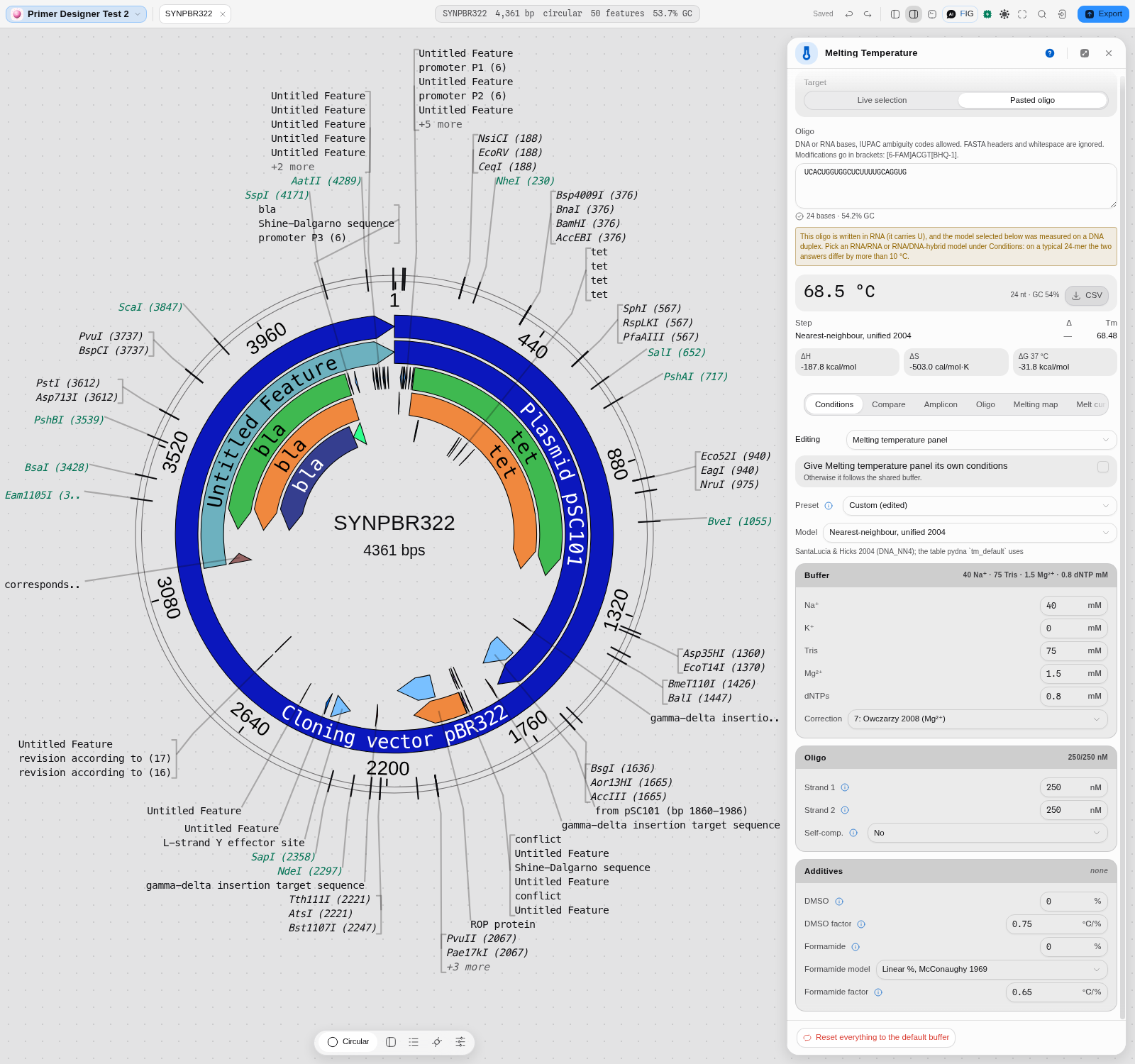
If you paste a sequence written with U while a DNA model is selected, the panel tells you before you trust the number, and the same warning fires the other way round. Switching the model clears it.
One thing the warning cannot catch: an RNA sequence written without any U in it — ACGACG is a
perfectly good RNA — looks exactly like DNA. Nothing in the letters says otherwise, so if you work
in RNA, set the model yourself rather than relying on the check.
The science
Every model is a port checked against its source implementation, from Biopython
(Bio.SeqUtils.MeltingTemp), pydna and QUEEN, plus the Teselagen models that came with the
editor. The panel selects among them and reports what each honours; it computes nothing itself.
Nearest-neighbour models sum stacking enthalpies and entropies over each adjacent base pair, add initiation and terminal terms, and solve for the temperature at which half the duplex is annealed at the stated strand concentration. That is why concentration appears at all, and why the four NN tables disagree: they were measured by different groups under different conditions.
The salt corrections are the published ones by name, and the additive corrections are Biopython's
chem_correction, and checked against it byte for byte.
One deliberate divergence from a source is worth knowing about: Biopython's own documentation states one DMSO factor while its code uses 0.75 °C per percent. The code is what was ported, because the code is what every downstream tool actually agrees with.
Shared with other tools: Melting temperature compares how every tool that does this chooses its method.
Limitations
- The Wallace rule is offered and is wrong above about 14 bases. It is included because real protocols and older tools still use it, and because comparing against it explains a discrepancy you may be chasing. On the 20-mer above it happens to land at 60 °C, close to the NN answer by coincidence rather than by agreement. It is the same rule that produces the misleading junction "Tm" in the Gibson panel.
- Betaine and glycerol corrections are not offered at all. Biopython has none, and betaine is isostabilising: its effect is non-linear and GC-dependent, with no single agreed conversion from percentage to ΔTm. Adding a plausible-looking factor would put a fabricated number into a temperature a user takes to the bench, so the fields are absent rather than approximated. This is a registered research gap: it needs an authoritative source (Rees 1993, Henke 1997) and its own validation oracle before it ships.
- The models disagree, and this tool does not pick a winner. It shows the spread and names the source of each so the choice is yours and is attributable. If you need one number, use the preset matching your polymerase's vendor and stay with it.
- The melting map and the melt curve are PREDICTED, not measured. They are what the Poland–Scheraga model says a molecule of this sequence should do in this buffer, and they carry that model's assumptions: no bound protein, no supercoiling, equilibrium at every temperature. A real instrument trace can differ, and where it does, the instrument is right. For fitting real amplification and melt data, that is the qPCR tools.
- A predicted curve has no noise, so its fine structure is real but not necessarily meaningful. Small −dθ/dT peaks are genuine features of the model rather than instrument artefacts, but a peak at 2 % of the tallest is not a domain anyone would resolve experimentally. That is what the smallest-peak filter is for, and why its default hides the smallest ones rather than pretending they are all equally interesting.
- Corrections are applied in the order the sources define, salt inside the model and additives after. A different ordering gives a slightly different total; this one matches the upstream libraries the ports are validated against.
Compared with other tools
Every claim about another product comes from the open claim register — first-party and dated 2026-08-08.
| jane* | SnapGene | Geneious Prime | |
|---|---|---|---|
| Tm as a first-class surface | Yes — model, buffer, strand concentration and additives are all controls | Not listed as a separate feature; Tm appears inside the primer tools | Not listed separately; appears inside primer design |
| Models offered | 8, each named with its citation | Not published | Not published |
| Salt-correction methods | 8, published ones by name | Not published | Not published |
| Additive corrections | DMSO and formamide, broken out per correction | Not published | Not published |
| Primer design that uses them | Primer Designer, sharing these exact conditions | Primer design and automatic primer design for cloning procedures | Primer design that also identifies off-target binding sites |
Read that table carefully, because "not published" is not "absent". Both products certainly
compute a Tm — it is inside their primer tools. What their public feature pages do not state is
which model, under which buffer assumptions, with which salt correction. We have not run either
product, so this page says what their documentation says and stops there (DOCS-RULES.md §5: never
call a competitor's science wrong unless you have run it).
What Geneious does here that we do not: its primer design automatically identifies additional off-target binding sites. Ours does not, in the Tm panel or the designer.
The difference that is real and checkable is not the count of models but where the number comes from: each of ours is checked byte for byte against the real Biopython, pydna or QUEEN function, with the source clone kept on disk so the vectors stay regenerable. That is a claim you can audit in this repository rather than take on trust — and it is the only claim on this page we can make about ourselves that we cannot check about anyone else.
Export
The computed Tm, the correction breakdown and the thermodynamic terms are readable in the panel and copyable. There is no dedicated file export from this panel: the number's destination is usually another tool in the editor, and because the conditions are shared, it gets there as a condition rather than as a pasted value.
The Primer Designer, which does export, carries these conditions into its own output.
API
import { tmNN, DNA_NN4, additiveCorrection, nnThermodynamics } from '@ports/tm';

const taq = {
  nnTable: DNA_NN4,
  Na: 40, K: 0, Tris: 75, Mg: 1.5, dNTPs: 0.8,
  saltcorr: 7,
  dnac1: 250, dnac2: 250, selfcomp: false,
};

tmNN('GTAAAACGACGGCCAGTGAA', taq);              // 61.48
nnThermodynamics('GTAAAACGACGGCCAGTGAA', taq);  // { tm, dH, dS, dG }
additiveCorrection(61.48, { DMSO: 5 });         // 57.73
Also exported: tmDefault, tmDbd, tmbresluc, tmProduct, taDefault, taDbd, tmGc,
tmWallace, tmNeb, saltCorrection, program and dbdProgram (cycling programs), and the four
DNA_NN* tables. resolveTmFunc turns a chosen model into the TmFunc other engines take, which
is how one buffer reaches every tool.
Everything is pure and synchronous. Temperatures are °C, concentrations are mM for ions and nM for strands, matching Biopython.
The whole-molecule melting behind the map and the curve is a separate entry point, because it is a different calculation rather than another Tm model:
import { meltCurve, derivativeCurve, meltTransitions, tm50, positionalHelicity } from '@ports/melt';

const temps = [80, 82, 84, 86, 88, 90];

const theta = meltCurve(plasmid, { temps, ions: 0.2 });   // fraction paired at each temperature
const rate  = derivativeCurve(plasmid, { temps, ions: 0.2 });

tm50(temps, theta);              // the 0.5 crossing, or null if it never crosses
meltTransitions(temps, rate);    // the melting domains: temperature, height, share of the tallest
positionalHelicity(plasmid, [84], 0.2);  // per-BASE pairing probability — what the map draws
tm50 returns null rather than a clamped endpoint when the temperature range never reaches half
melted, and meltTransitions reports interior maxima only, so the edge of the range you asked for is
never returned as a domain.
Automation
The conditions are shared state rather than a per-run argument, so automation mostly consumes them
rather than setting them: a workflow node that designs or checks primers computes with whatever
TmFunc the conditions produce.
There is no standalone tm node in the workflow DAG and no dedicated copilot tool for it. That
is a real gap rather than a design decision, and it means a workflow cannot currently state the
buffer it wants. Calling @ports/tm directly is the way to do it in code.
Provenance
The conditions are part of the editor's shared state, so a run that used them is reproducible when they are recorded alongside it. Each preset states its source string, and the panel shows every correction as its own line, so a number can be traced back to model plus buffer plus additive rather than appearing as a bare temperature.
The corrections breakdown is the citable part: it names which published method produced which degrees.
Screenshots
The melting map is captured — two temperatures on the same real plasmid, in The melting map, in full above: 75 °C (mean helicity 0.994, 8 domains) and 88 °C (0.054, 9 domains), showing that the only thing that moved was the temperature.
The melt curve is captured in The melt curve above, and one more frame belongs here because it is the only one showing the two views working as a pair:
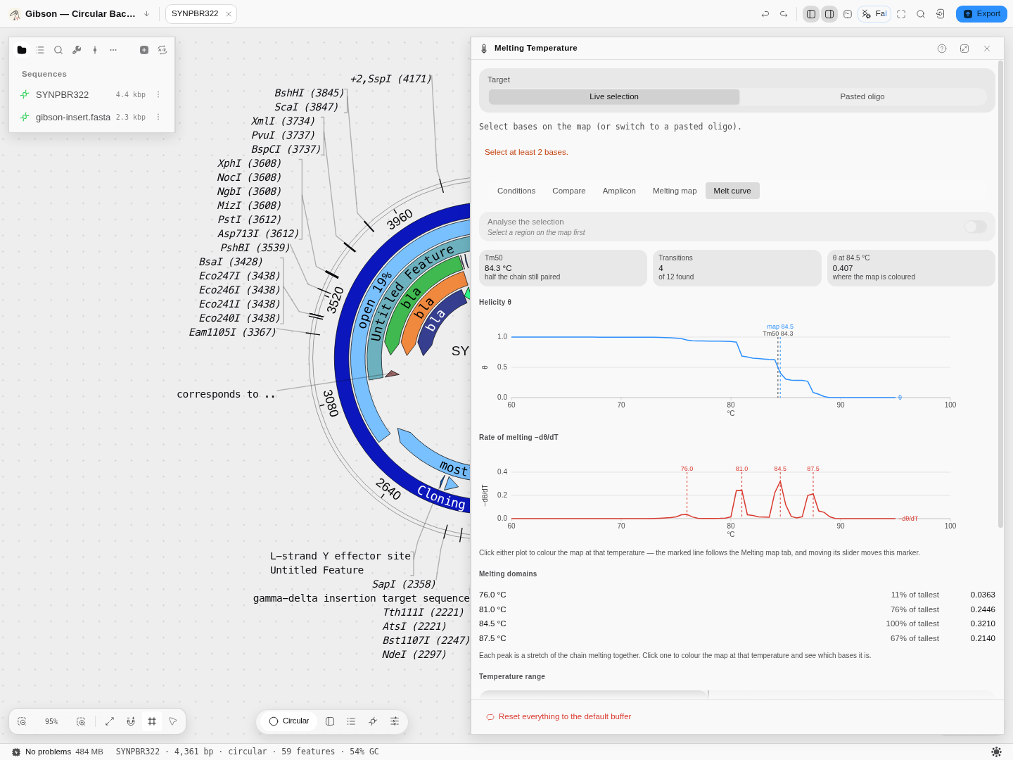
pBR322 after clicking the 84.5 °C domain in the melt curve's domain list — the tallest peak. The marker's helicity has fallen from 0.984 to 0.407 and the map, still painted on the tab behind, has recoloured to match. That is what the two views sharing one temperature buys you.
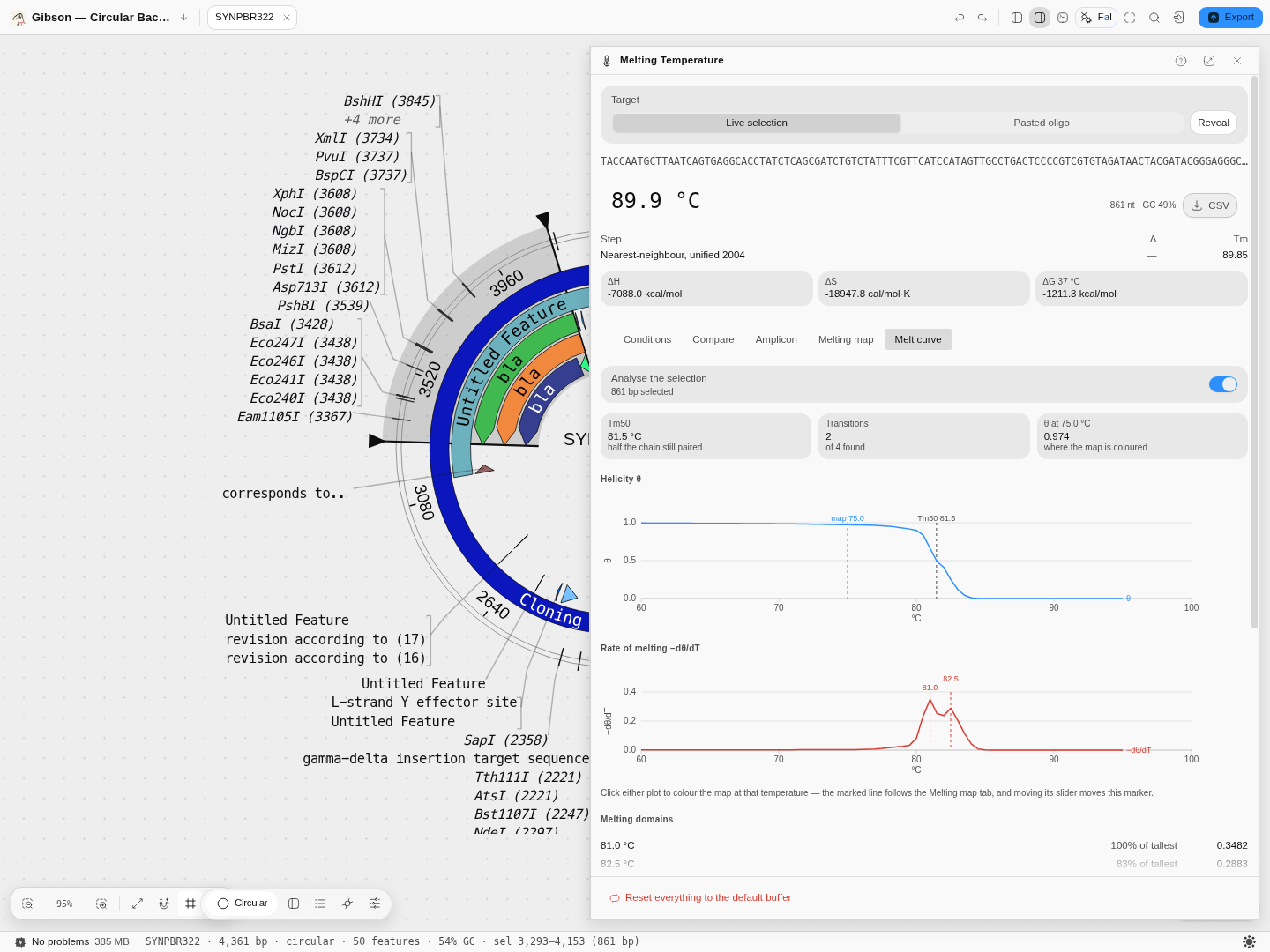
The same plasmid with the analysis restricted to the 861 bp bla CDS: Tm50 81.5 °C over two
domains, against 84.3 °C and four for the whole plasmid — one gene melting more simply than the
molecule containing it. Note the oligo readout above the tabs reads 89.9 °C for the same bases:
that is the two-state nearest-neighbour model, which is the wrong question at this length, and the
8.4 °C gap between the two numbers is the clearest illustration on this page of why both exist.
Still to capture: the conditions form with the disabled fields visible, which is the frame that shows a model stating what it ignores.
Related
Feeds it: any selection on the canvas, and the Primer Designer, whose candidates are scored with these conditions.
Follows it: PCR Simulation and its thermocycler program, which derive annealing temperature from these models; Mutagenesis, which selects primers on Tm; qPCR, for real curve and melt data.
Compare with: the Gibson panel's junction Tm, which is the Wallace rule and is not comparable to these numbers.
Droplet classification
Sort droplets into their populations: two targets under three methods that disagree, or up to four targets by density, spectral clustering, flow peaks or the consensus of all three.
Codon Optimization
Rewrite a coding sequence for expression in a chosen host while holding the constraints that matter: forbidden restriction sites, GC window, homopolymer limits, and the encoded protein.