
Codon Tables
Marked experimental: the surface can change.
A codon optimisation is only as good as the usage table behind it.
| Reached by | Tools → Codon Tables |
| Formats | CDS FASTA in (plain or gzipped) Codon usage TSV in and out |
| Sample project | Codon usage |
What it does
Every codon-usage number you can compute — CAI, Fop, %MinMax, an optimisation — is a comparison against a reference table: how often each of the 61 sense codons is used, in some set of genes, in some organism. Codon Tables is where that reference comes from when a published one will not do. It counts a table from real coding sequences you supply, or reads one someone else counted, and then makes it available to every other codon-aware tool as an ordinary host.
It counts. It does not model, weight or smooth anything: a codon's number is the number of times it appeared in the sequences you gave it.
When you’d use this
Used in: Optimize a coding sequence for expression in another host
Reach for it when the organism you care about is not one of the bundled 36, when the published table is too old to trust, or when "the organism's codon usage" is the wrong question and you need a narrower set of genes than a whole genome.
- Your expression host is not in any catalogue — a new isolate, an engineered strain, a chassis nobody has deposited. You have its annotated genome; that is enough.
- The published table is frozen. Kazusa is fixed at the 2007 GenBank release. If the organism's reference assembly has been re-annotated since, counting the current CDS set yourself gives a different — and more defensible — table.
- You want the highly-expressed genes, not the genome. Codon-adaptation indices were defined against a highly-expressed reference set, not against all genes (Sharp & Li 1987). Those two tables can disagree sharply in a biased genome, and a CAI computed against the wrong one is quietly measuring something else.
- You want to compare a construct against a specific gene set — a pathway, an operon, a set of well-expressed reporters.
What this computes
It counts. It does not model, weight or smooth anything — a codon's number is the number of times it appeared in the sequences you gave it.
- Per-codon counts and their synonymous share within each amino-acid family, over the 61 sense codons, from a real CDS corpus you supply — or read from a table someone else counted
- The corpus behind the number: how many CDS records were counted, how many of them were the gene set you asked for, the total codons, how many of the 20 amino acids are represented, and GC3 — the third-position GC, which is the composition summary a bias measure is usually judged against
- Two gene sets, which are different references: highly-expressed counts only the ribosomal-protein genes — the classic reference set for "what does this organism use when it means it" — and the genome mode counts every CDS in the file
- The genetic-code chart the table is read under, in
RNA (U)orDNA (T)notation, with each cell carrying its codon, amino acid and synonymous usage percentage within its own family
A table you count here becomes an ordinary host everywhere else — the codon-usage measures, the optimizer, back-translation. User tables are namespaced, so one cannot silently shadow a bundled reference host; a name collision stays two distinct tables rather than becoming one wrong one.
What it does not compute: whether the table is a good reference. A table counted from four genes is arithmetic just as valid as one counted from four thousand and describes almost nothing — which is why the corpus size is a readout rather than a footnote.
Where it lives
Tools → Codon Tables. It is a workbench tool rather than a document view: it does not read the open sequence and it does not draw on the map, because a usage table is a property of a reference set, not of the construct you happen to have open. What it changes is what the other tools can choose: a table saved here appears as a host in Codon Usage Analysis, the Codon Optimizer and Back-translate.
Inputs and outputs
In, one of two shapes.
- A CDS FASTA — one record per coding sequence, each in frame from its first base. NCBI's
cds_from_genomic.fnaalready has exactly this shape, so an organism's whole CDS set is one download. Accepts.fna, gzipped.fna.gz, and pasted text. - A codon-usage TSV — a table someone else counted, as codon/count columns.
Out: a saved table with its build statistics, exportable as TSV, and registered as a host for every codon-aware tool in the workbench.
What it refuses, and how. An empty paste is declined by name before anything runs ("Paste a CDS FASTA first" / "Paste a codon-usage TSV first"), and an unreadable file names the file and the reason. Records whose length is not a multiple of three are truncated to the last whole codon rather than dropped or padded — a trailing partial codon is not evidence about codon usage, and neither is a guess at what it would have been. Fetching a genome directly from NCBI, or mirroring Kazusa, is not offered here; the panel says so rather than showing a control that fails.
Demo
Open the Codon usage sample project, then Tools → Codon Tables → Try a sample. The corpus is real and bundled, so nothing is fetched.
Worked example
M. genitalium, from the bundled corpus — data/samples/CDS/Mycoplasma_genitalium_NC_000908.2_cds.fna,
the NCBI RefSeq CDS set for NC_000908.2.
-
Tools → Codon Tables. The panel opens on From CDS FASTA with Highly-expressed selected.
-
Click Try a sample · M. genitalium ribosomal-protein genes. The corpus loads and the table builds in one step.
-
Read the build statistics. 524 CDS total, 52 of them highly expressed, 6,990 codons counted, 20/20 amino acids present, GC3 30%.
The two counts are the point: the table you just built rests on 52 genes, not 524. That is the correct reference set for a codon-adaptation index, and it is also small enough that the panel tells you the count instead of leaving you to assume it.
-
Read the genetic-code chart. Every codon with its amino acid and its synonymous share — the percentage within its own amino-acid family, so the four alanine codons sum to 100 and not the whole table.
RNA (U)switches the display toDNA (T); the numbers do not change. -
Export or spend it. TSV downloads the table. Sending it to the optimizer registers it as a host, and it then appears in Codon Usage Analysis and Back-translate under the same name.
A run over the whole genome instead of the ribosomal-protein set is the same three clicks with Highly-expressed switched to the genome mode, and comparing the two GC3 figures is the fastest way to see whether this organism's expression bias is real.
Controls
| Control | What it changes |
|---|---|
| Build route | From CDS FASTA counts codons from sequences · From codon-usage TSV reads a table someone else counted |
| Gene set | Highly-expressed counts only the ribosomal-protein genes · the genome mode counts every CDS in the file |
| Table name | The host name the table takes everywhere else. Optional; user tables are namespaced so one cannot silently shadow a bundled reference host |
| CDS corpus | Paste, or From a file… for .fna / .fna.gz / .tsv |
| Genetic-code chart | The code the chart is displayed under, and RNA (U) / DNA (T) notation |
| TSV | Downloads the saved table |
Algorithms you can choose
One selection rule, and it is a rule rather than a model. The highly-expressed set is chosen by
what the FASTA headers say the genes ARE: a record counts as highly expressed if its header names a
ribosomal protein, or carries an rpl / rps / rpm gene tag. Ribosomal-protein genes are the
canonical highly-expressed reference set — the one Sharp & Li used to define CAI — because they are
translated at high rates in every growing cell, so their codon choices track what the tRNA pool
actually supplies.
Two details that are deliberate and would be wrong the other way:
- Transferases are excluded even when they say "ribosomal protein".
rimIandprmAmodify ribosomal proteins; they are not ribosomal proteins, and they are not highly expressed. A header match that ignored this would quietly dilute the reference set. - The highly-expressed table is never backfilled from the genome. If an amino acid never appears in the 52 genes, the table says so instead of borrowing that row from the whole-genome counts. A backfilled row would be a per-codon repair spliced in from a different gene set, and there is no coherent way to say what set the resulting table came from. This is what the 20/20 amino acids readout is for: it tells you whether the reference set was large enough before you use it.
Beyond that there is nothing to choose, because there is nothing to estimate — the table is counts.
The science
A codon-usage table is a contingency table: for each amino acid, how its synonymous codons were divided in a set of genes. Everything downstream is a normalisation of it. Relative adaptiveness w = f/fmax within each family. CAI is the geometric mean of w over a coding sequence. RSCU is the observed count over the count expected if the family were used uniformly.
The choice that matters is which genes are in the set, and it is not a detail. Sharp & Li defined the index against highly-expressed genes precisely because those are the ones under translational selection; a whole-genome table also carries mutational bias, horizontally-transferred genes and everything that is expressed rarely. In an organism with strong translational selection the two tables disagree, and the disagreement is the biological signal — which is why this tool reports the gene counts for both and keeps them separate.
GC3 — GC content at third codon positions — is reported next to them because it is the fastest check on whether a table's bias is translational or compositional. A genome whose GC3 is extreme has codon "preferences" that are mostly mutational, and a CAI against it is measuring base composition.
Counting conventions, stated because they change the numbers. Sequences are read in frame from
the first base, uppercased, U mapped to T. Non-standard codons are not counted. Only whole
codons are counted. Raw counts, never derived fractions, are what get registered for other tools to
use — the registry re-normalises within each family under its own genetic code, and handing it a
fraction column would normalise twice.
Shared with other tools: Codon usage compares how every tool that does this chooses its method.
Limitations
- It counts what you give it. The tool cannot tell a mis-annotated CDS, a pseudogene or a frame-shifted record from a real one. Garbage in the corpus is garbage in the table, and the only guard is the statistics it reports back — the CDS count, the amino-acid coverage and GC3.
- The highly-expressed rule is a header rule. It reads annotation, not expression data. On a corpus with sparse or non-standard headers it will find few genes or none, which the counts will show; on a genome where ribosomal-protein genes are unusual it is the wrong proxy.
- No genome fetch and no Kazusa mirror from this panel. Both are deferred rather than stubbed. Get the CDS FASTA yourself, or use the live NCBI and Kazusa sources in Codon Usage Analysis.
- A small reference set gives a noisy table, and a CAI against it carries that noise. The 52-gene sample above is a realistic ribosomal-protein set for a minimal genome; it is also close to the point where the amino-acid coverage readout starts to matter.
Compared with other tools
Not yet written as a comparison. Establishing what each incumbent does today would need its own documentation read with a retrieval date, and that has not been done for this tool — so rather than characterise other people's software from memory, this section says only what can be said without a source, which is about this panel.
Two things here are unusual enough to be worth stating plainly. The first is that the gene set is a control rather than an assumption: most places that hand you "the codon usage of X" hand you one table and do not say which genes are in it, and the highly-expressed and whole-genome tables of the same organism are different tables answering different questions. The second is that a table you build is a first-class host everywhere else — not a file you re-import per tool, but a name that appears in the analysis, optimisation and back-translation panels alike, resolved through the same registry as the bundled references, with raw counts rather than a re-normalised fraction column.
API
Panel-only today. Unlike the codon-usage analysis, building a table is not yet exposed to the in-app Python and R consoles or to the workflow builder — the same counting engine is behind both, checked against the CUTG release the tables come from, but nothing calls it from outside the panel. Building a table is a handful of clicks and its output is reusable everywhere once saved, so this is a convenience gap rather than a capability one; it is named here so nobody plans a pipeline around a route that does not exist.
Automation
Not scriptable yet, for the reason above. To build tables for many organisms today, run the panel once per corpus; each saved table persists and is selectable by name afterwards, so the downstream work — scoring, optimising, back-translating against those tables — automates normally through the codon-usage and optimiser steps.
Export
TSV of the saved table, per table. The table also leaves the panel as a host rather than as a file: registered once, it is selectable in Codon Usage Analysis, the Codon Optimizer and Back-translate under the name you gave it.
Provenance
A saved table records the route it was built by and the gene set it used (CDS · HEG or
CDS · genome), the CDS and codon counts behind it, its amino-acid coverage and its GC3. Those five
numbers are what a methods section needs: a table is only reproducible if the reader knows which
genes were counted, and how many.
To cite the method: state the assembly accession of the CDS set, the gene set (highly-expressed ribosomal-protein genes, or all CDS), and the number of CDS and codons counted.
Screenshots
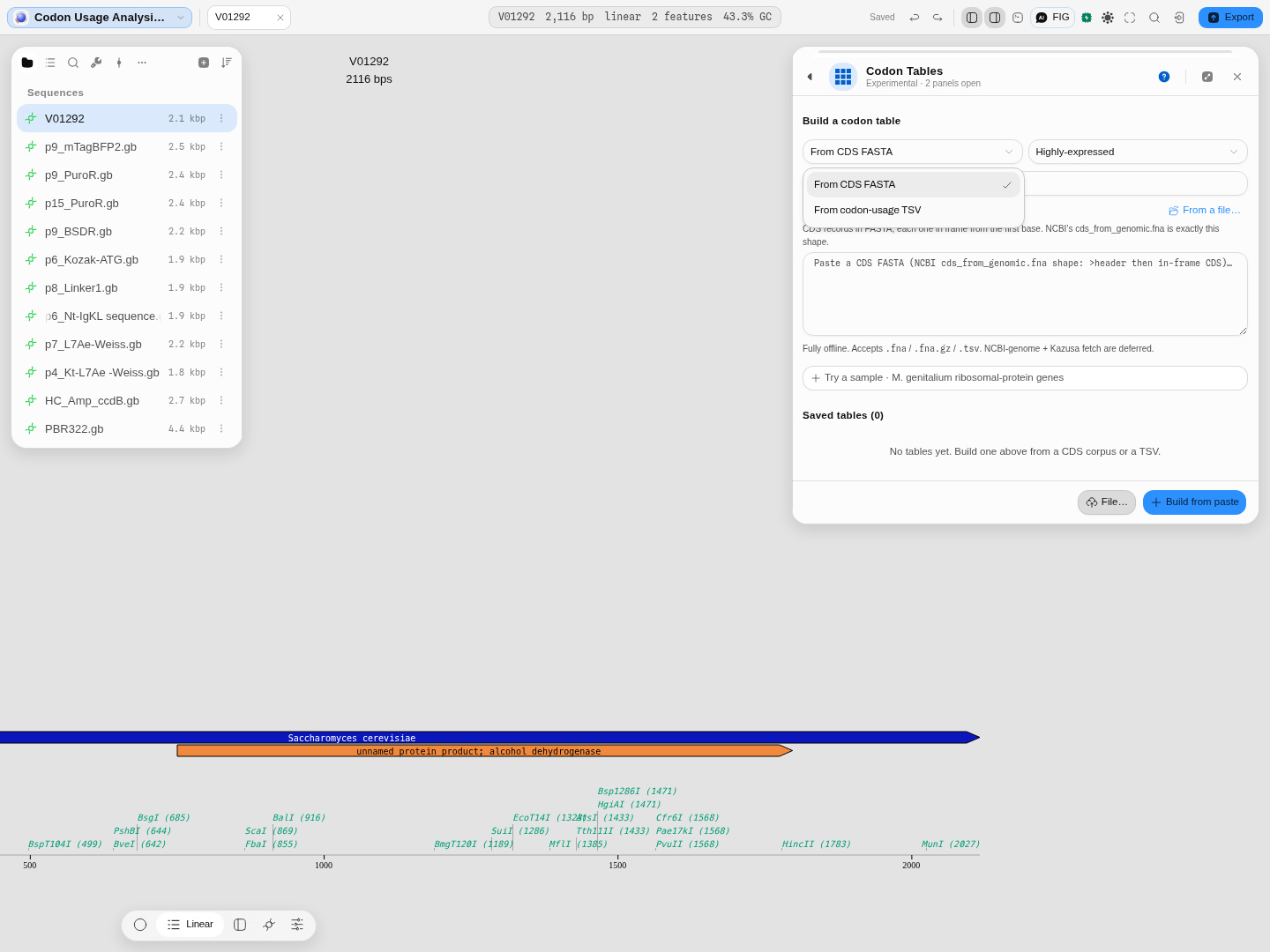 Two build routes: a CDS FASTA — the shape NCBI's
cds_from_genomic.fna already has — or a codon-usage TSV. Both run entirely on your machine.
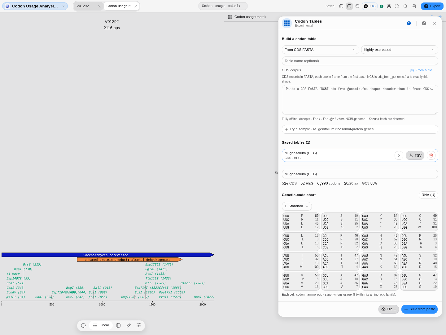 The M. genitalium ribosomal-protein sample, counted: 524 CDS, 52 of them highly expressed, 6,990 codons, all 20 amino acids present, GC3 30%. The chart shows every codon with its synonymous share within its own amino-acid family, in RNA notation.
Related
In this group: Properties · BLAST Search · Search Databases · EMBL-EBI Services · Protein Domains · Protein Analysis · Protease Digest · Antibody Numbering · Mass spectrometry: peptide masses, b ladders, isotopes, spectrum scoring, q-values, protein inference · Codon Usage Analysis · Site avoidance: restriction sites a genome avoids or favors · Codon outliers: genes whose codon usage departs from their own genome · Tree incongruence: genes whose own alignment rejects the species tree · Reference stability: reference genes against genes of their own abundance · Annotation contradictions: UniProt features a predictor scores unlike confirmed ones · Hypothesis ledger: pre-register a hypothesis, attach runs, decide with e-BH · Reagent audit: does each annotated CDS code for what the map says, and are its cryptic promoters, splice sites and repeats worse than chance · Assay decay: does a published assay still match current genomes, and is the mismatch at the 3′ end · Gene incongruence: which loci of a multi-locus alignment have a different history · Target validation: test "gene G drives phenotype P" against gene-level evidence tables · Enzyme Collections · Virtual Gel Bench · Phylogenetics · Dot Plot · Table · NumPy Array · Structure · PDF · Molecule · Image
Target validation: does a gene drive a phenotype
Test a gene–phenotype hypothesis against gene-level evidence tables with POPPER's sequential falsification and e-values.
Enzyme Collections
The enzyme list, scoped to the sequence you have open: every enzyme carries how many times it cuts this construct, Type IIS enzymes are flagged as cutting outside their recognition site, and the collection you make here is the one the digest tool offers.