
Protein Analysis
Read the physicochemical properties of a protein the way ExPASy ProtParam does, without leaving the editor or pasting a sequence into a form.
| Reached by | Tools → Protein Analysis |
| Sample project | Protein tools |
What it does
Translates a coding region from the construct you have open and reports what the protein it encodes would actually be: its mass, its charge, how stable it is likely to be in a cell, how much light it absorbs at 280 nm, and where along the chain it is hydrophobic, amphipathic or charged.
These are the ProtParam quantities — the ones on every protein datasheet — computed on the record in front of you rather than on a sequence you pasted into a web form and now have to keep in sync.
When you'd use this
Used in: Optimize a coding sequence for expression in another host · Protein → peptides: will mass spectrometry see the region I care about? · Read a variant call set at a locus
Before you order or express anything. The extinction coefficient is how you will quantify the protein once you have it, and the isoelectric point decides whether the purification buffer you planned will keep it soluble.
When an expressed protein behaves badly. An instability index above 40, a GRAVY that says the chain is more hydrophobic than you assumed, or a pI sitting on your buffer's pH are all visible here before you spend a week on inclusion bodies.
When you need the number an instrument will report. Average mass and monoisotopic mass are both shown, and they are different numbers — the second is the one to compare against a mass spectrometer.
When you are choosing where to put a tag or a mutation. The Profile and Amphipathicity tabs say which stretches are buried, exposed or membrane-like, so a tag goes somewhere it will not disrupt a fold.
Reach for something else when: you want the peptides a protease would produce — that is Protease Digest; or you want to know which domains the protein has — that is Protein Domains.
What this computes
Every readout the panel produces, named the way it is searched for.
Whole-molecule quantities. Average molecular weight and monoisotopic mass (the one a mass spectrometer reports); theoretical isoelectric point on the Bjellqvist pKa set; net charge at any pH from 0 to 14, with the full titration curve; molar extinction coefficient at 280 nm in both the reduced and the cystine-containing form, and the A280 of a 1 g/L solution for each; instability index; aliphatic index; grand average of hydropathicity (GRAVY), on any of 28 hydropathy scales — including transfer free energies and hydrophilicity scales, which run in the opposite direction, so each GRAVY is reported with the end of its scale that is the hydrophobic one, and on a scale whose values never cross zero no hydrophobic/hydrophilic verdict is given at all; aromaticity; Boman potential protein-interaction index; maximal Eisenberg hydrophobic moment at both the α-helix and β-sheet periodicities; atomic composition as a molecular formula and an atom count; and estimated in-vivo half-life in mammalian reticulocytes, yeast and E. coli from the N-end rule.
Residue composition. The count and the percentage of the chain for every amino acid, absences included as explicit zeros, ordered by abundance; the acidic (D+E) against basic (K+R) balance that carries the isoelectric point; the cysteine count and whether it is even, which decides how many disulfides can form; and the elemental composition behind the molecular formula, each element with its share of the atom count. All of it readable as a chart and takeable as a table.
Per-residue profiles, each windowed and plotted along the chain, over 71 published ProtScale scales — hydropathy, hydrophilicity, transmembrane tendency, surface accessibility, backbone flexibility, antigenicity, bulkiness, polarity, refractivity, recognition factors and the rest — with any of six offered as a one-click overlay against the one you are reading, under either of ProtScale's two window weighting models, linear or exponential. Alongside them: the windowed hydrophobic moment, and predicted secondary-structure fraction (helix, turn, sheet).
Predictions with a stated method. Transmembrane topology by a class hidden Markov model, decoded by Viterbi, posterior-Viterbi, optimal-accuracy or N-best, giving per-residue inside / outside / membrane assignment, the helix count, the side of the membrane each terminus is on, the decoder's own score in the form that decoder reports it, and the mean posterior probability the model placed on the labels it actually chose. The same decode drawn as a membrane snake plot, one circle per residue across the bilayer, colored by compartment, by any hydropathy scale or by side-chain charge at a pH; with the lysine and arginine count on each side of the membrane (the positive-inside rule), and, where the record carries curated transmembrane annotations, how many of their residues fall inside a predicted helix. Signal-peptide cleavage position by the von Heijne weight matrix, scored per position, for either the eukaryotic or the prokaryotic matrix. Intrinsic disorder two ways: by metapredict, a neural network trained to reproduce a consensus of disorder predictors, giving a 0–1 disorder score for every residue, the intrinsically disordered regions (IDRs) and folded domains its domain caller draws, and the percentage of residues at or above its threshold, from any of its three published networks (V1, V2, V3); and by FoldIndex and Uversky's charge–hydropathy boundary, per window and over the whole chain.
Interpretation, generated from the run. What the numbers say together: whether the molecule is net positive or negative at your working pH and which ion exchanger will therefore bind it, whether it sits near its solubility minimum, whether the instability index clears the bar the method publishes, what the composition's acidic/basic balance does to the pI, which residues are absent and what their absence costs, and how reliable an A280 measurement will be for this particular chain.
On the cleavage-site scan: where the cut falls and what mature chain it leaves, whether that position is somewhere a signal peptide could actually be, how far the winning site beats its nearest rival, which of the fifteen scored positions carried the score and which one argued against it, and — where the open record carries its own signal-peptide annotation — whether the prediction and the curator agree, and by how many residues if they do not.
On disorder by metapredict: how much of the chain scores disordered, how many IDRs the domain caller draws and how much of the chain they cover, the longest one and its mean score, how many residues sit close enough to the threshold that the call could go either way, whether FoldIndex agrees residue by residue and on the whole protein, and which nonstandard residues (selenocysteine, X, B, Z) had to be read as a standard one first.
On disorder by FoldIndex: the whole-chain score against the charge–hydropathy boundary it was judged by, with the distance from that line; how many windows fall on the disordered side and where the longest run of them is; and a warning when the whole-chain score and the window scan point in opposite directions, which is what a rigid protein with locally disordered-looking composition produces.
On every windowed profile: which residue the highest and lowest windows fall on, the mean across all of them, how many windows sit above zero on a signed scale, and — when scales are overlaid — how far apart they peak, compared by position rather than by value, because the scales are in different units.
Uncertainty and refusal, stated rather than implied. A quantity that cannot be computed is withheld with the reason, never approximated: a residue with no entry in a hydropathy table blocks GRAVY and the instability index rather than being silently dropped from the sequence, an ambiguous letter is counted in the length but left out of the mass, and a protein with no tryptophan is told that its extinction coefficient may be more than 10% out.
Where it lives
Tools → Protein Analysis opens it in the right rail. Right-click a CDS on the map → Protein analysis opens it already scoped to that feature. Whatever you select on the canvas, the panel follows.
It writes back to the canvas too: the Amphipathicity tab's Show these runs on the map draws the transmembrane, surface-seeking and globular runs along the sequence, so "where is the membrane helix in my construct" is answered on the map rather than in a list.
Inputs and outputs
Accepts any annotation on the record, an open reading frame it finds for you, a canvas selection or pasted residues. DNA is translated first, under a genetic code you choose; a protein record is read directly.
The annotation list is ordered, not filtered: entries typed as coding — CDS, gene, ORF, protein
— come first, and every other annotation follows, each row naming its own type and strand. That
matters on a well-annotated record, where a tRNA gene, an rRNA gene and the whole-record source
entry all sit in the same list as the CDS you want; and it matters on a sparsely typed one, where
the coding regions may be recorded as misc_feature and would vanish from a list that filtered by
type. Nothing is hidden from you, and nothing is presented as coding that the record does not say
is coding.
Refuses in words, before it computes anything. A region that is not a whole number of codons says how many trailing bases it would ignore. A frame running through internal stop codons says how many there are — "54 internal stop codons in these residues — this frame runs through them, so the readouts describe a protein that is not translated" — and offers the longest genuine reading frame instead, as a button. Non-standard residues are counted in the length but excluded from mass and GRAVY, and the panel says which numbers that leaves undefined rather than printing a plausible one.
Produces the summary tiles, seven further tabs of detail — composition, profile, amphipathicity,
disorder, topology, signal peptide and charge — the map overlay, and Copy / FASTA / CSV of the
residues and the values. Every one of those readouts can equally be asked for in words, with the
same parameters and the same defaults you see on the controls.
Demo
Not recorded yet. The screencast worth making is the Profile tab: change the scale and watch the same protein tell a different story. Nothing is staged in the meantime.
Worked example
eGFP, read out of the vector that carries it. Open the Protein tools sample project
(CVU55762 — cloning vector pEGFP-N1, 4,733 bp circular) and pick Feature → egfp · 720 bp · CDS.
The header confirms egfp (720 bp) → 239 aa before any number appears.
| eGFP | |
|---|---|
| Length | 239 aa |
| Average mass | 26.94 kDa (26,941.15 g/mol) |
| Monoisotopic mass | 26,924.4834 Da |
| Isoelectric point | 5.58 (Bjellqvist) |
| Instability index | 29.05 — stable (≤ 40) |
| Aliphatic index | 79.04 (Ikai 1980 — thermostability) |
| GRAVY | −0.467 (Kyte & Doolittle) |
| Boman index | 1.63 kcal/mol (≤ 2.48 — membrane-selective) |
| Aromaticity | 10.0 % (Lobry 1994 — F+W+Y) |
| ε₂₈₀, reduced | 21,890 M⁻¹cm⁻¹ · A280 at 1 g/L = 0.813 |
| ε₂₈₀, all cystines | 22,015 M⁻¹cm⁻¹ · A280 at 1 g/L = 0.817 |
| Net charge at pH 7.0 | −7.70 |
The two numbers to carry away: an A280 of 0.813 for a 1 g/L solution is how you will read the concentration off a spectrophotometer, and a pI of 5.58 means this protein is negatively charged at physiological pH — which is why it binds an anion exchanger and why it will aggregate if you buffer it near pH 5.5.
The reduced-versus-cystine pair is a real choice, not a rounding difference. eGFP has 2 cysteines, so the two coefficients differ by 125 M⁻¹cm⁻¹ — small here, and not small on a disulfide-rich protein. The panel exposes which convention it is counting under.
Controls
The tabs, and what each is for
| Tab | The question it answers | When you would not open it |
|---|---|---|
| Summary | "What is this protein, on a datasheet?" It opens on the hydropathy profile, then mass, pI, stability, GRAVY, extinction coefficient | Never — it is the tab you check first |
| Composition | "What is it made of?" Every residue with its count and percentage, ordered by abundance | When the question is positional rather than compositional |
| Profile | "Where along the chain is it hydrophobic / flexible / accessible?" A sliding-window plot over a scale you choose | On a very short peptide, where a 9-residue window leaves almost no curve |
| Amphipathicity | "Does it have membrane-like or surface-seeking stretches?" The hydrophobic moment, and the runs it implies | On a protein you already know is soluble and globular |
| Disorder | "Which parts of this chain are likely to have no fixed structure at all?" metapredict's per-residue score with its IDRs and folded domains, or the FoldIndex curve with the runs that fall below zero and where the whole protein sits on the charge–hydropathy plane | On a protein you only need a global answer for — the Summary tab's GRAVY already says how hydrophobic it is overall |
| Topology | "Which residues are in the membrane, which side is each loop on, and how sure is the model?" Every residue assigned to inside / membrane / outside in one pass, with the helix count, the orientation of the N-terminus, a choice of four decoders and a confidence beside every run | On a protein with no membrane-like stretches at all — the Amphipathicity tab will have said so first |
| Signal | "Where would signal peptidase cut, and what mature protein would that leave?" Ranked cleavage sites, and the mature chain each implies | On a protein you know is cytosolic — though running it is a useful negative |
| Charge | "How does its charge behave with pH?" Net charge at a pH you set, and the whole titration curve | When the pI on the Summary tab is all you needed |
The knobs, and what each does to the number
| Control | Effect |
|---|---|
| Target — Feature · ORF · Selection · Paste | What is analysed. An ORF is found for you and listed longest-first with its frame |
| Genetic code | The translation table. Changing it changes the protein, so every number moves. Shown only when there is DNA to translate |
| ε₂₈₀ cysteine convention | Whether cysteines are counted as free thiols or as cystines (per disulfide, or per residue). Identical unless the cysteine count is odd |
| Hydropathy scale (GRAVY) | Which published scale GRAVY averages, out of 28. It changes the number and can change the verdict: bacteriorhodopsin, a seven-helix membrane protein, reads +0.72 (hydrophobic) on Kyte & Doolittle and −0.18 on the Engelman transfer free energy — the same molecule, because the two scales run in opposite directions. The panel says which end of the scale you chose is the hydrophobic one, so the sign is never read on its own |
| Profile → Scale | Which of the published amino-acid scales the curve is drawn from — hydropathy, flexibility, accessibility and others. The curve's meaning changes with it, so the axis label carries the scale's name and citation |
| Profile → Window | How many residues are averaged per point. Larger smooths the curve and hides short features; smaller is noisier and shows them |
| Profile → Edge weight | How much the residues at a window's edges count relative to its centre, from 1.0 (flat) downward |
| Profile → Weight variation | How the weight falls from the centre to the edge weight. Linear steps down evenly. Exponential falls steeply next to the centre and flattens toward the edges, so the curve follows the central residues more closely and sharp features survive a wide window. At an edge weight of 1.0 the two are identical |
| Profile → Normalise to 0–1 | Rescales the scale's twenty values before windowing — which is what makes two different scales comparable on one axis. It does not rescale the finished curve |
| Amphipathicity → Window / Angle | The moment's window, and the rotation per residue: 100° is an α-helix, 160° a β-sheet. A helix and a sheet give different answers on the same sequence, and both are offered |
| Amphipathicity → Min. windows / Class | How many consecutive windows of one class make a run, and which classes are listed. Raising it drops short, noisy runs |
| Show these runs on the map | Draws every listed run on the sequence. Highlights only — the record is never modified, and they clear when the panel closes |
| Color residues by (Topology) | Compartment, Hydropathy or Charge: what the snake plot paints each residue with. Its assigned side of the membrane, its value on the scale the Profile tab is set to (the same numbers the profile plots, so it is unavailable on a non-hydropathy scale such as Vihinen flexibility), or its side-chain charge at the Charge tab's pH. It recolours the picture only; the topology call does not change |
| Signal → Eukaryotic / Prokaryotic | Which of the two published training sets the cleavage matrix is built from — 161 eukaryotic or 36 prokaryotic aligned signal peptides. The same sequence scores differently under each, so pick the one matching where the protein is actually made, not where the gene came from |
| Signal → Minimum score | Only sites scoring above this are listed. At 3.5 the method finds about 95% of real signal peptides and rejects about 95% of non-signal sequences; lower it to see near-misses, raise it to keep only strong calls |
| Charge → pH | The pH at which net charge is reported. The curve beside it shows every other pH at once |
The graphs, and how to read them
Profile — hydropathy (or another scale) per window. The x axis is residue position, 1-based, at the centre of the window; the y axis is the scale's own units, averaged over the window, and it is labelled with both. On eGFP with Kyte & Doolittle at window 9 the curve runs from −3.46 to 2.33: values above zero are hydrophobic stretches, below zero hydrophilic. What you are looking for is shape, not height — a sustained plateau above ~1.6 across 19 or more residues is the classic membrane-helix signature; a spiky curve crossing zero every few residues is an ordinary soluble protein, which is what eGFP is.
Comparing scales on one axis. Compare with overlays up to four further scales on the same plot, which is how you tell a real feature from a property of the scale you happened to pick: a stretch that reads hydrophobic on Kyte & Doolittle, inaccessible on the accessibility scale and high on transmembrane tendency is a membrane segment; one that moves when you change scales is an artefact of the scale. The scales are in different units and share one axis, so turn on Normalise to 0–1 before reading their shapes against each other — the panel says so under the buttons.
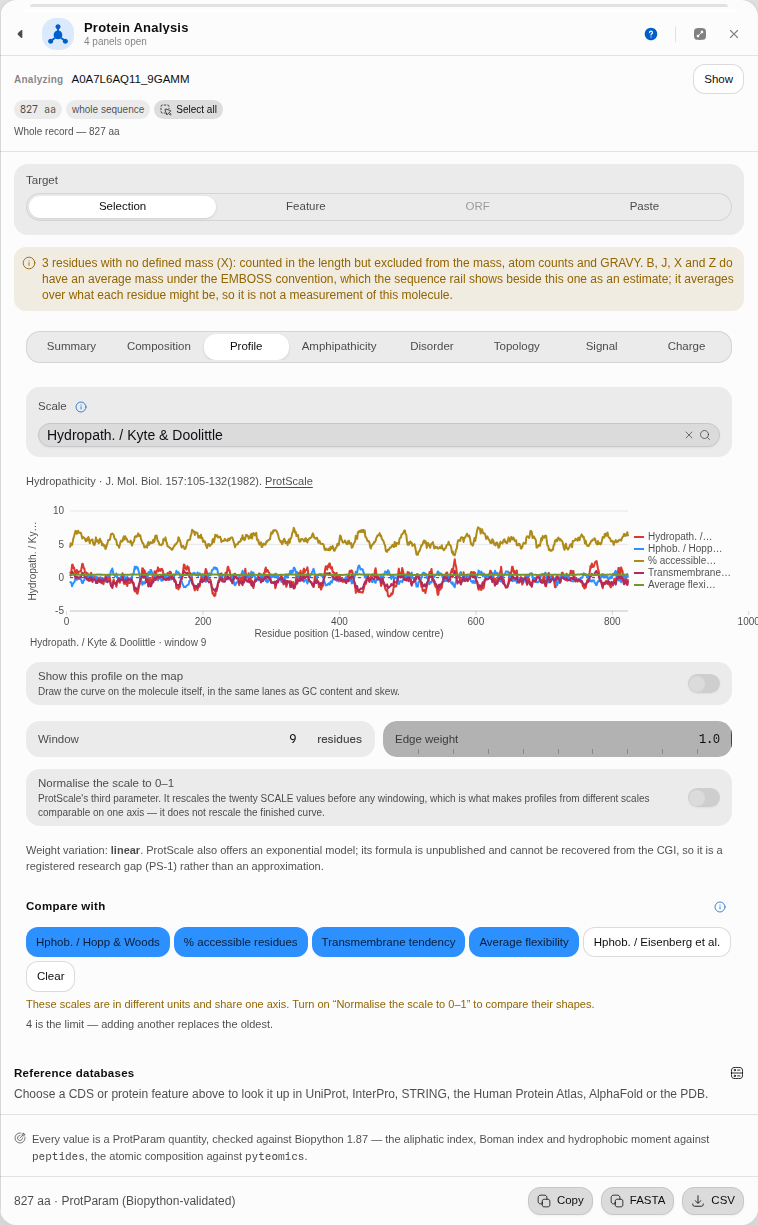 The primary scale plus four overlays. Every curve is also named in the key beside the plot, so the comparison survives greyscale printing and colour-vision deficiency; four is the limit, and adding a fifth replaces the oldest rather than crowding the axis further.
Amphipathicity — the hydrophobic moment μH per window. Same x axis; y is μH, which measures how one-sided the hydrophobicity is when the chain is wound at the angle you chose. High μH with moderate hydropathy means an amphipathic helix — one face oily, one face polar — which is what membrane-interacting and surface-seeking segments look like. eGFP peaks at μH 0.651 (α-helix, 100°) and 0.885 (β-sheet, 160°); the sheet number being the larger one is consistent with a β-barrel, which is what eGFP is.
The membrane strip, under the plot. One coloured cell per window — 254 windows of 11 residues on eGFP — classified Globular (233), Transmembrane (7) or Surface-seeking (14). Point at it to read a window; use the arrow keys to walk it; press Enter to select that window on the map. It is the compressed version of the two curves above, and the fastest way to find the stretch worth looking at.
Charge — the titration curve. x is pH, y is net charge in elementary charges, and the curve crosses zero exactly at the pI. On eGFP it spans +36.00 to −47.94 and crosses at 5.58. The useful reading is the slope at your working pH: a curve that is steep there means small pH drifts change the protein's charge a lot, which is a buffering problem before it is a chromatography problem.
The rest, by name
| Control | Default | What it sets |
|---|---|---|
| Residues or coding DNA | empty | A sequence pasted in instead of the open record |
| Scale | Hydropath. / Kyte & Doolittle | Every scale ExPASy ProtScale publishes, plus the Biopython tables it does not |
| Normalize the scale to 0–1 | off | ProtScale's third parameter. It rescales the twenty scale values before any windowing, which is what makes profiles from different scales comparable on one axis; it does not rescale the finished curve |
| Edge weight | 1 | How much a residue at the window's edge counts against one at its center |
| Weight variation | Linear | How that weight falls off. Linear steps down evenly; Exponential is ProtScale's second model, decaying steeply near the center |
| Min. windows | 2 | How many consecutive windows must pass before an amphipathic run is reported |
| Minimum score | 3.5 | The weight a signal-peptide site must reach to be reported |
| Net charge model | Counted charges · K + R − D − E (Prilusky 2005) | Counted charges, or fractional charges at pH by Henderson-Hasselbalch. The two answer different questions, and the paper only settles the first |
| pH | 7 | The pH the charge is computed at |
| pKa set | IPC_protein | Fifteen published sets. The same window's charge moves by more than a full unit between them, so the set is part of the answer |
| Count histidine as positive | off | At pH 7 histidine is about 9 % protonated, so Uversky counts K and R against D and E. Some later tools include it |
Finding a signal peptide, step by step
Secreted and periplasmic proteins are made with an N-terminal signal peptide that a signal peptidase cuts off during export. Knowing where that cut falls tells you the mature protein's real mass, its real pI, and — if you are cloning — where a tag can go without being thrown away with the leader. This walkthrough uses pBR322's β-lactamase, which is a textbook case, and you can check every number against the record itself.
1 · Open the construct and pick the coding sequence. Open the Protein tools sample project
and select PBR322.gb. Set Target → Feature and choose bla · 861 bp · CDS (−). The header
confirms bla (861 bp, reverse strand) → 286 aa before anything is computed. The gene is on the
minus strand, which is worth noticing: everything below is reported in residues, and the panel maps
those back to the right bases for you.
2 · Open the Signal tab and choose the matrix. β-lactamase is made in E. coli, so press Prokaryotic. The note under the buttons tells you what you just chose — 36 aligned prokaryotic signal peptides — and the two matrices genuinely disagree: this same protein scores 7.6 against the eukaryotic one and 10.5 against this one.
3 · Read the top site, and the sentences under it. The best site is after residue 23, score
10.527, leaving a 263-residue mature chain beginning HPETLVKV…. Five sites clear the
default threshold of 3.5; the other four score 5.2 and below and sit deep in the chain.
Under the two tiles the panel takes that score apart, because a single number over a fifteen-residue window hides most of what it is made of:
- where the cut is, and — if it falls past residue 70 — that a real signal peptide is almost never cleaved that far in. The bound is not a guess: across every reviewed Swiss-Prot entry that carries a signal peptide, 99.9% are cleaved at or before residue 70, and the median is 22. The matrix itself has no notion of position, so on a long protein its best-scoring window is routinely a look-alike rather than a signal peptide, and the panel says which of the two you are looking at;
- how isolated the call is: here it beats the next site by 5.31, out of five above the threshold. A site that wins by a hair is a different result from one that stands alone;
- which residues carried it:
V at -3 (+0.18) and A at -1 (+2.27) carry 2.45 of the 10.53 total. Those are the two positions signal peptidase reads most closely, and this is where you see the classic small residue at −1 doing the work; - which one argued against it: the most negative of the fifteen weights, named with its position. A total is a sum, and a sum hides a residue that is voting the other way.
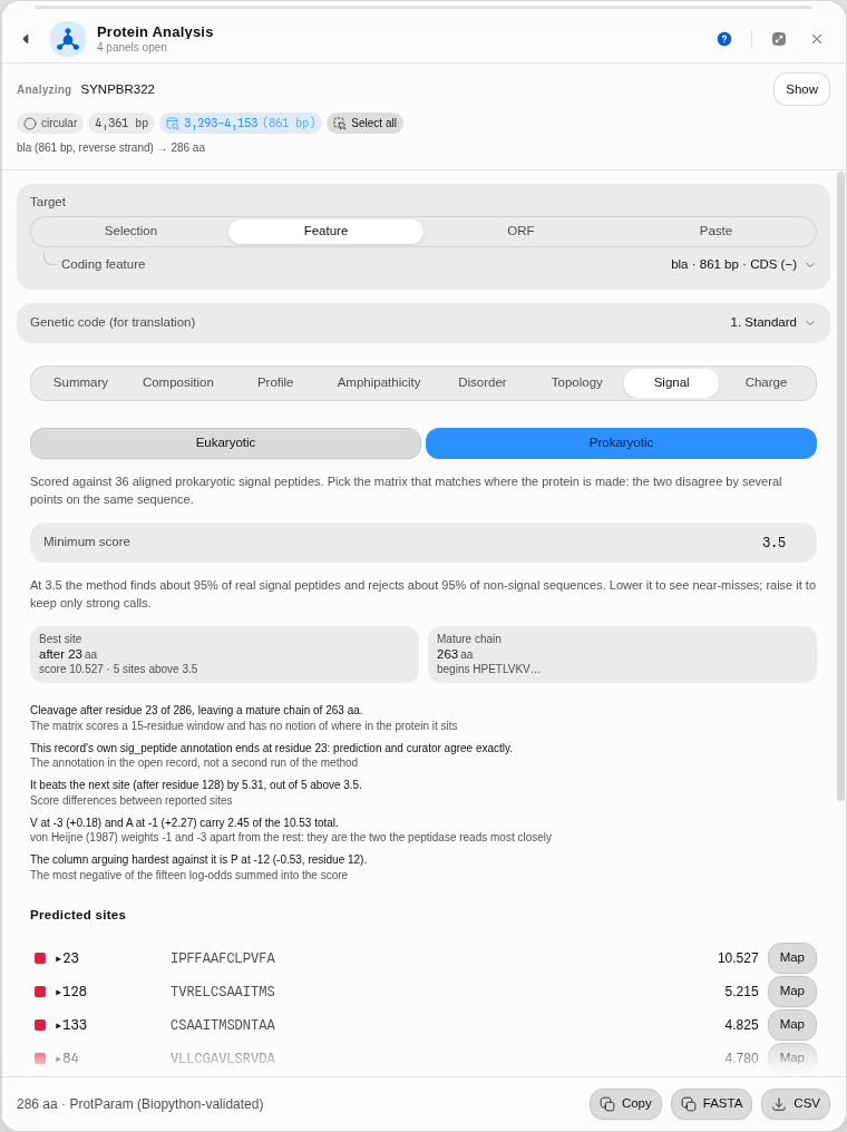 Step 3, with step 4 already done: cleavage after residue 23, and the peptide drawn on the circular map.
4 · Draw it on the map. Press Map beside the top site. Two spans appear on the sequence — the signal peptide 1–23 and the mature chain 24–286 — and you can see them in the circular map's label stack. They are highlights, not edits: nothing is written to the record, and they clear when the panel closes. Clicking the row itself instead selects just the 13 scored residues.
5 · Check it against the record — the panel already has. pBR322's GenBank entry was curated
independently of any prediction, and it carries a sig_peptide feature on bla of 69 bp (23
codons) and a mat_peptide of 789 bp (263 codons). Those are exactly the two numbers the panel
produced, and it says so in the reading: "This record's own sig_peptide annotation ends at residue
23: prediction and curator agree exactly."
That line appears whenever the open record carries its own signal-peptide annotation, and it is worth understanding what it is not: it is the annotation already in the file, not a second run of the method, so it is an independent check rather than a confirmation of the panel by itself. Where the two differ, the reading gives the distance in residues instead of a verdict. Where the record has no such annotation — as with GFP below — the line simply does not appear.
6 · Run the negative control. Switch to CVU55762 and target egfp. GFP is cytosolic; it has
no signal peptide, and the method must not invent one. The best site comes back at residue 209 of
239 — deep in the back half of the chain — and the panel says so in as many words rather than
presenting it as a find.
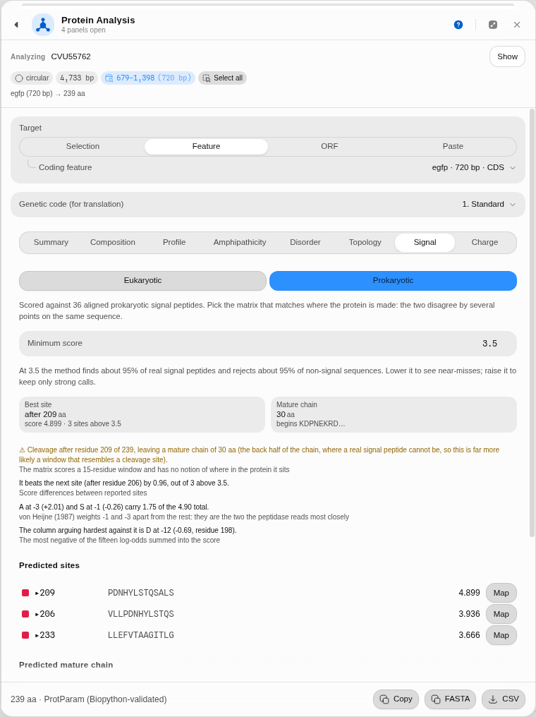 Step 6. The tile is deliberately not coloured as a positive result, because a mid-chain site is not a signal peptide.
6b · The same thing on a protein record. The walkthrough above starts from DNA, but the most
direct case is a protein entry that carries its own annotation. In the same project, open
P01308.txt — human preproinsulin, 110 residues, the hormone's precursor. No target needs choosing:
the whole record is the protein. The eukaryotic matrix puts the cut after residue 24, which is
exactly where the entry's own curated signal peptide ends, and the next two sites (18 and 15) are
there to show what a near-miss looks like. The residues at −3 and −1 are both alanine — the
Ala-X-Ala pattern that turns up again and again at real cleavage sites, here recovered from the
weights rather than looked up in a list.
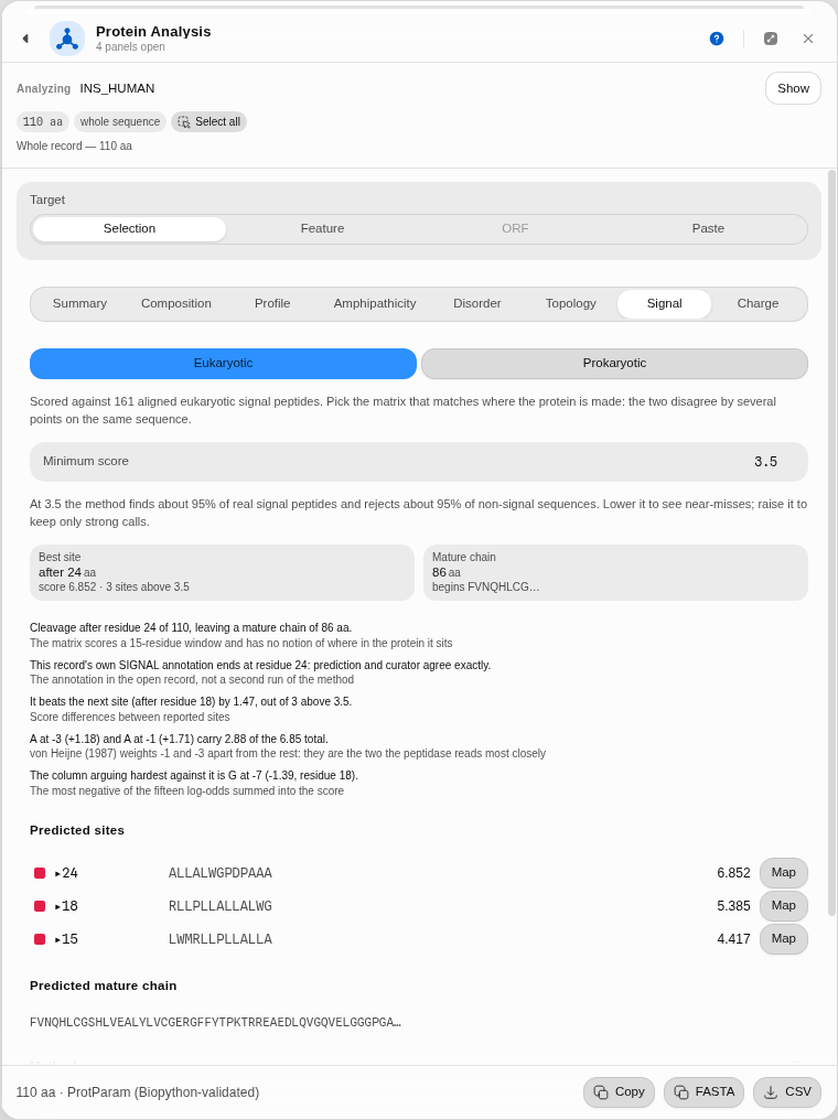 Step 6b. The prediction and the curator agree on residue 24, and the panel says which is which.
7 · What happens with residues it cannot score. Set Target → Paste and enter a sequence
containing X, B, Z or U. The tab refuses, names each letter with what it stands for, and
counts the affected positions. It does not score around them — a window missing one of its fifteen
terms would produce a number that looks fine and is not.
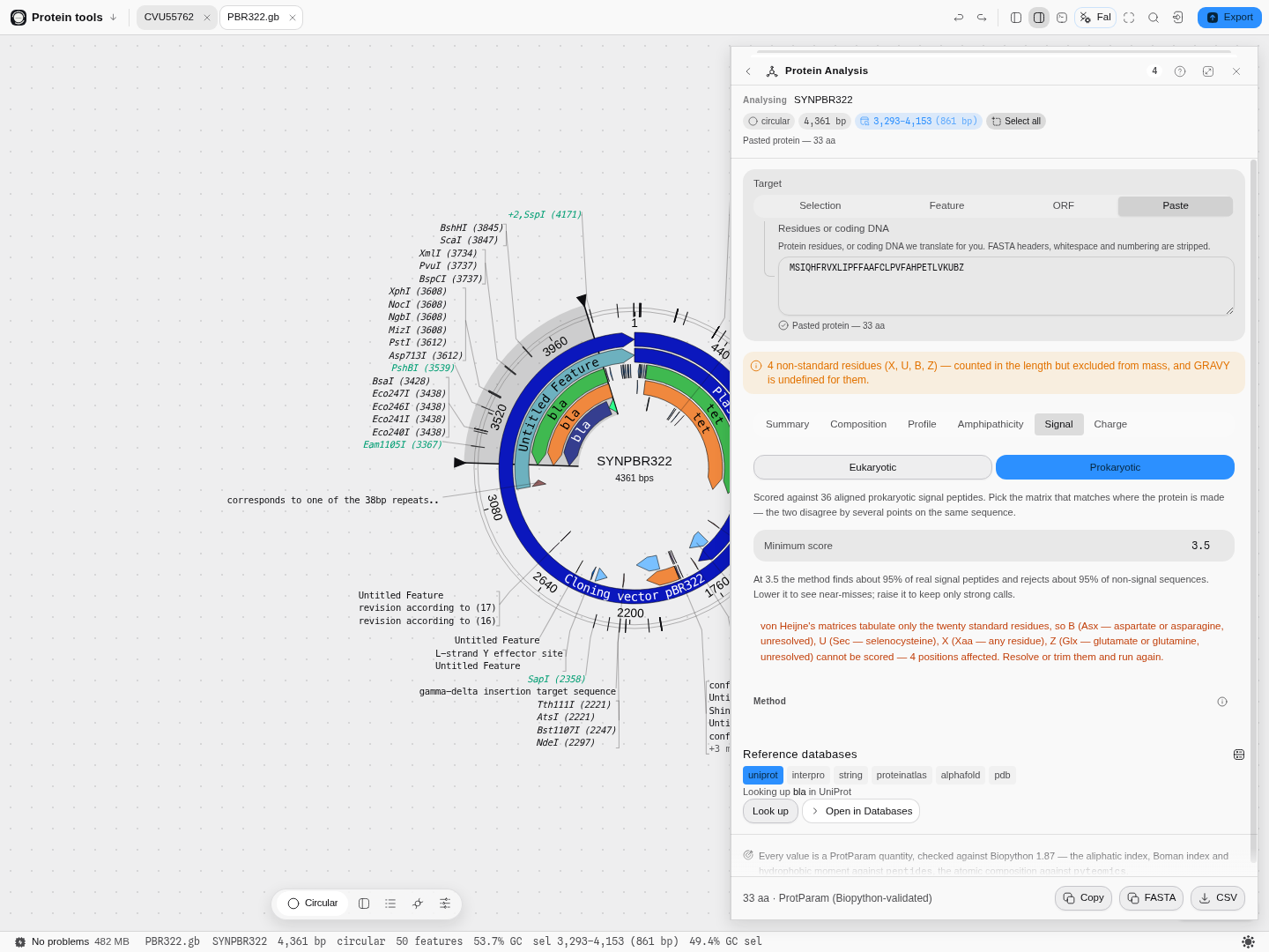 Step 7. Ambiguity codes and non-standard residues are refused by name, not silently skipped.
How the method works, and where it stops
The matrix looks at a fixed 15-residue window around every possible cut: the 13 residues before it and the first two after. Each residue at each position carries a log-odds weight — how much more often it appears there in real signal peptides than by chance — and the site's score is the sum of the fifteen. Positions −1 and −3 are treated specially, and that is the point of the method rather than a detail: signal peptidase reads those two positions closely, so a residue never observed at them is penalised heavily instead of merely scoring low. This is why the classic small-residue pattern at −1 and −3 dominates the result.
What it answers: where the cut would fall. What it does not answer: whether the protein is secreted at all. The matrix sees a 15-residue window and has no idea where in the chain that window sits, which is exactly why GFP produces a mid-chain hit. Treat a high score near the N-terminus as a cleavage-site prediction, and a high score elsewhere as a sequence that happens to look like one.
Pitfalls worth knowing:
- The matrix must match the expression host, not the gene's origin. A eukaryotic gene expressed in E. coli should be scored prokaryotic if the question is what the bacterium will do to it.
- The score is not a probability. 10.5 is not "94% confident"; it is a sum of log-odds. Use it to rank candidate sites within one protein, and use the 3.5 threshold as the published operating point.
- A protein with no site is a real answer. Most proteins are cytosolic. An empty list at 3.5 is information, not a failed run.
- The training sets are from 1986 and are small — 161 and 36 sequences. The method is durable and still the standard weight-matrix approach, but it is a statistical pattern over a few hundred proteins, not a model of the enzyme.
Algorithms you can choose
The Profile tab is the catalog: each entry is a published amino-acid scale with its own citation, shown on the axis when selected, so a curve can always be attributed. Kyte & Doolittle hydropathy (J. Mol. Biol. 157
–132, 1982) is the default because it is the one most protocols and papers mean by "hydrophobicity plot".The Profile tab can also draw its curve on the molecule, not just beside it: Show this profile on the map puts the windowed scale into the same concentric ring and row lane that GC content and GC skew use, spanning only the coding region you analysed. It is worth turning on when you are looking for where on the construct a hydrophobic stretch falls relative to a restriction site or a tag, which the plot's own residue axis cannot tell you. It is a view: it clears when you close the panel and is never written into your file.
The hydrophobic moment offers the two periodicities that matter — 100° for an α-helix and 160° for a β-sheet — because they answer different structural questions, and neither is a better version of the other.
The extinction coefficient offers the two cysteine conventions, and the isoelectric point is the Bjellqvist calculation, named on the tile.
The disorder prediction offers two definitions of net charge, and they are different questions
rather than a setting and its fallback. Counted charges is what the FoldIndex paper specifies —
lysine and arginine minus aspartate and glutamate, divided by the window length. Fractional charges
at a pH titrates every ionisable group through Henderson–Hasselbalch instead, so histidine, cysteine
and tyrosine each contribute a fraction, against any of fifteen published pKa sets. The same window's
charge moves by more than a full unit between IPC_protein and Rodwell, which is why the set is
named on the panel rather than chosen for you. Histidine is a third open question inside the first
model — at pH 7 it is about 9% protonated, so the classical set leaves it out — and it is a switch.
The signal-peptide scan offers von Heijne's two matrices — eukaryotic and prokaryotic — as a real choice rather than a default, because they are built from different training sets and disagree on the same sequence.
Reading a membrane protein's topology, step by step
Hydropathy tells you where a stretch looks membrane-like. It cannot tell you which side of the membrane the loop between two helices is on, because it looks at one window at a time and a compartment is a property of the whole chain. The Topology tab answers the second question: every residue assigned to inside, membrane or outside, decoded in one pass under a grammar where a helix must be followed by a loop on the opposite side of the bilayer.
That constraint is the whole method. It is why a topology model can tell you your C-terminal tag will end up in the periplasm, and why a hydrophobicity plot never can.
Open the Protein tools sample project and follow along on pBR322 — its tetracycline-resistance gene encodes TetA, a textbook 12-pass transporter.
-
Open
PBR322.gbfrom the Files rail. -
Target the
tetCDS. In Protein Analysis choose Feature, thentet · 1191 bp · CDS. The header should readtet (1191 bp) → 396 aa. -
Open the Topology tab. The first line is the reading: "12 transmembrane helices; N-terminus inside." That is TetA's published architecture — twelve membrane-spanning segments with both termini in the cytoplasm — recovered from the sequence alone.
Under it, the reading spells out what the call rests on: the helix ranges, which side each terminus is on and therefore whether a terminal tag lands in the same compartment at both ends, and the mean posterior probability the model put on the labels it chose. That last number is the one to read before trusting the rest — a topology can be drawn confidently and still be marginal, and a low mean is the model saying so.
-
Read the runs. Below it, all 25 compartment runs in order, each with its residue range and length:
Inside 1–4,Transmembrane 5–25,Outside 26–40, and so on. The loops are listed as well as the helices, deliberately — the alternation is the topology, and a list of helices alone would not tell you the orientation. -
Switch on Show the topology on the map. The coding region is now tiled by compartment on the circular map, and in the linear and sequence views: blue for membrane, green for inside, orange for outside. Hovering any run gives its range and the model's log probability for the whole path.
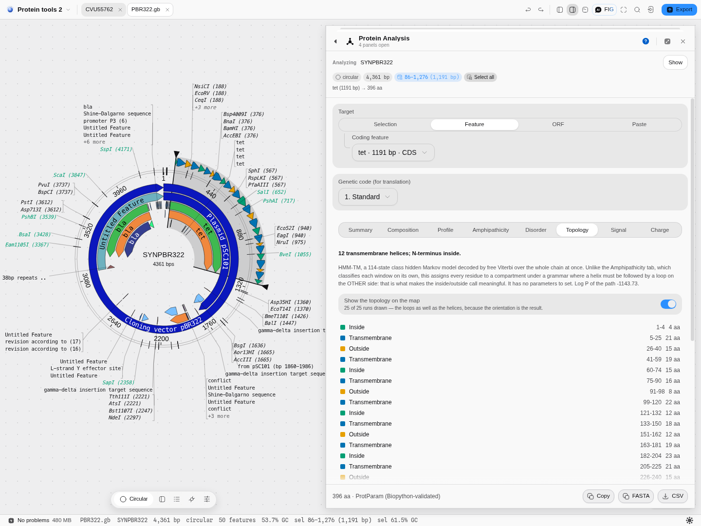
-
Click a run to select exactly those codons on the map — useful when you are choosing where to insert a tag or a protease site and need somewhere that is not buried in the bilayer.
Which decoder, and how sure the model is
A topology model does not produce one answer. It produces a probability distribution over every possible assignment of every residue, and a decoder turns that into the single picture you read. Four are offered, and they answer four different questions:
| Decoding | What it maximises | When to reach for it |
|---|---|---|
| Viterbi | The probability of the path as a whole | The default, and what this model's published results are reported on. Use it unless you have a reason not to |
| Posterior | The best path through per-residue probabilities | When you care that each residue is called correctly and the exact chain of transitions matters less |
| Best accuracy | The expected number of residues called correctly | When you want the assignment most likely to be right residue-by-residue, even if that path is individually less probable |
| N-best | The best whole LABELLING, summing over every state consistent with it | When you want the labelling itself scored rather than a path through the model's internal states. It is the slowest by far — a second or two on a long chain — and on this benchmark the closest to Viterbi |
They are not four settings for one answer. On the reference method's own 72-protein benchmark, Posterior moves the call on 34 proteins, Best accuracy on 46 and N-best on 9. Switching decoder is a scientific choice, so it is on the panel rather than buried.
The score under the picture is not comparable between decoders, and it is not a quality mark. Each decoder reports the quantity its own method defines: Viterbi gives the chosen path's log-probability, which is read against the whole-sequence log-likelihood printed beside it; N-best gives a score already divided by that likelihood, so it sits near zero; and the two posterior decoders sum log per-residue probabilities and subtract the sequence likelihood, which comes out positive and is not a probability of anything. A bigger number is therefore not a better answer, and the same protein legitimately scores -760, +582, +760 and -4.6 under the four. Compare a score only against another run of the same decoder — to judge the answer itself, use the percentage below.
Beside every run is a percentage: how much probability actually sat on that call, averaged over the run's residues. This is the number that tells you whether to believe the picture, and it is the thing a single best path structurally cannot give you.
Two cases, both in the sample project, show why it matters:
-
Bacteriorhodopsin (
P02945in the Files rail) is the textbook seven-helix membrane protein. All four decoders call seven helices, N-terminus outside, and every run reads 78–98%. That is what a clear-cut answer looks like — and because this record carries its own curated membrane annotations, they draw on the map directly beneath the prediction, so you can see the agreement rather than take it on trust. Every predicted boundary lands within three residues of the curated one.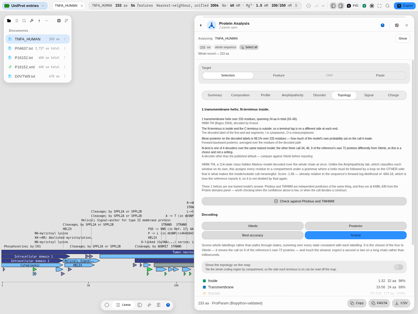
Under the reading, the tab draws the chain across the membrane: each helix crosses it, each loop hangs on the side the decoder put it, and a dark ring marks every residue the record's own curation puts in a membrane span. On bacteriorhodopsin 128 of the 135 curated residues fall inside a predicted helix, and the rings show you where the other seven are: at helix ends, which is where curation and prediction usually part. Color the residues by Hydropathy and the helices run hydrophobic through the bilayer while the loops do not; color them by Charge and you can count what the caption counts for you, 7 lysines and arginines on the inside against 4 on the outside. That excess on the cytoplasmic side is the positive-inside rule von Heijne described in 1986 for bacterial inner-membrane proteins, and it is the independent check on the orientation the model chose. Click any residue to select it on the map.
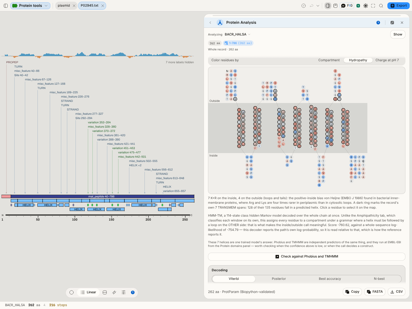
-
A marginal case looks completely different. On photosystem I subunit PsaL, Viterbi calls three helices and Best accuracy calls two, with the orientation flipped between them. The confidences say exactly why: the helix Viterbi adds carries 39% support, every run the two decoders disagree about sits at 34–39%, and the two helices both agree on read 93%. Without the percentages you would have two confident-looking pictures and no way to choose; with them, the disagreement is localised to the part of the molecule the model is genuinely unsure about.
The practical rule: a run in the nineties is a result. A run in the thirties is the model telling you it is guessing, and switching decoders will often move it.
What to check before you trust it
-
A single predicted helix is the one to distrust, and eGFP shows you why. Point the tab at the
egfpCDS in the same project — a cytosolic β-barrel with no membrane segment at all — and the model reports one transmembrane helix, over the last 21 residues. That is not a bug in this implementation: the reference gives the same answer, residue for residue. It is what a hydrophobicity-driven topology model does with a hydrophobic stretch at a chain terminus, and it is the single most common way these predictions mislead. Run it anyway — knowing that the method calls a helix here is worth more than a tool that quietly hides the case.The practical rule: one helix, at a terminus, on a protein you have no other reason to think is membrane-bound, is a hypothesis and not a result. Twelve alternating helices with consistent orientation, as on TetA above, is a result.
-
The N-terminal call has a second explanation worth ruling out. A signal peptide is hydrophobic and can be read as a first transmembrane helix by a model that does not know about signal peptidase. Run the Signal tab beside this one: if it puts a strong cleavage site inside what Topology called helix 1, treat the first segment as a signal peptide, not a membrane anchor. The two tabs disagreeing is information, not a bug.
-
This model reads the twenty standard amino acids and nothing else. Give it an
X, aBor aZand it refuses by name — residue number and letter — rather than substituting something. A substituted residue moves helix boundaries, and you would have no way of knowing it happened.
What we offer here that the incumbents do not
The web servers for this class of method take a pasted sequence and hand back a picture. Here the topology is computed on the construct you have open, its runs land on the same map as your features and cut sites, and clicking one selects the codons — so the answer is in the coordinate system you are actually cloning in. The runs are their own map track, with their own visibility switch and their own limit, so turning them on does not disturb the record's own annotations or its feature count. And it runs entirely on your machine: nothing about your construct leaves it.
And four decoders, not one. The incumbent servers pick a decoding for you and never say which; here you choose, and you see how much the choice moved the answer. The per-run confidence is not offered by the web servers for this method at all — they hand back a picture with no indication of which parts of it are marginal.
Provenance. The model is HMM-TM, a 114-state class hidden Markov model. All four decoders — Viterbi, posterior-Viterbi, the optimal-accuracy posterior decoder and N-best — are checked against the reference implementation residue for residue on all 72 proteins of its own published test set, 17,465 residues each, with their scores matching to six decimal places. The per-residue probabilities come from the same forward–backward pass the reference uses.
Finding disordered regions, step by step
Intrinsically disordered regions have no single folded structure. They are common in regulatory and signalling proteins, they are where many degrons, phosphosites and binding motifs live, and they are the usual reason a construct expresses well and then refuses to crystallise. The Disorder tab offers two predictors that answer the question differently, and each is a check on the other: metapredict (the default) and FoldIndex. Both run on your machine and need nothing but the sequence.
With metapredict
metapredict is a small bidirectional recurrent network trained to reproduce the consensus of several disorder predictors (Emenecker, Griffith & Holehouse, Biophysical Journal 2021). It scores every residue from 0 to 1, and its domain caller turns the profile into regions: it smooths the scores, calls a residue disordered above the threshold, closes short gaps and drops runs shorter than the minimum IDR size. Its output here is checked residue by residue against metapredict itself on more than 7,000 proteins, for all three networks.
The Predictor switch above the tab chooses metapredict or FoldIndex. Under Run settings, Network picks the trained model: V3 is the package default, V1 is the network the 2021 paper describes, and V2 and V3 are the lab's retrained successors. Threshold is the score a residue must exceed to be called disordered, left at the network's own value unless you set it. The domain caller's three lengths are metapredict's own defaults: Minimum IDR size (12 residues) is the shortest region reported as an IDR; Minimum folded domain (50) is the shortest stretch between two IDRs kept as folded, so a shorter gap whose mean score is above 0.75 of the threshold is absorbed into the IDRs around it; and Gap closure (10) fills short runs of sub-threshold residues flanked by disordered ones, so one dip does not split an IDR in two.
1 · Open a protein and go to Disorder. From the Protein tools sample, open P49908.txt
(selenoprotein P, 381 residues), select the whole sequence and open the Disorder tab.
2 · Read the profile against the dashed threshold. The curve is the per-residue score and the dashed line is the network's own threshold (0.5 for V3 and V2, 0.42 for V1). On selenoprotein P, 116 of its 381 residues score at or above it and the domain caller draws two IDRs, residues 1–36 and 193–272, covering 30.4% of the chain.
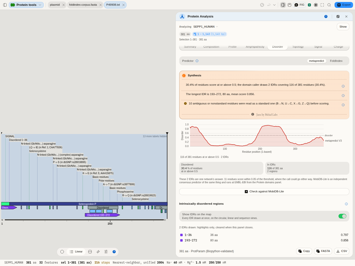 Selenoprotein P in the Disorder tab: two IDRs, drawn on the linear view. The second (193–272) lands on
the record's own "Disordered" region 200–268, which UniProt took from MobiDB-lite, an independent
consensus predictor. MobiDB-lite's other region (355–381) rises toward the threshold here but stays
under it, and the first IDR (1–36) contains the signal peptide (1–19), which is not disorder in the
folded protein.
3 · Read the caution about the residues. Selenoprotein P carries ten selenocysteines, and the network has inputs for the twenty standard residues only, so the reading says that ten residues were read as cysteine before scoring, the same substitution metapredict's own FASTA reader makes.
4 · Draw the IDRs on the map. Switch on Show IDRs on the map and every IDR appears as a violet span on the circular, linear and sequence views; clicking one in the list selects it.
5 · Change the knobs and watch the regions move. Network picks V3 (the default), V2 or V1 (the network the 2021 paper describes). Threshold defaults to the chosen network's own; Reset to the network's own restores it. Minimum IDR size is the shortest region reported and sets the smoothing window (twice it); Minimum folded domain decides when a short ordered gap between two IDRs is absorbed into them; Gap closure fills short sub-threshold runs flanked by disordered ones.
With FoldIndex
FoldIndex is the fast, fully explainable first look: a formula over charge and hydropathy. Switch Predictor to FoldIndex.
1 · Open a protein and go to Disorder. From the Protein tools sample, open
foldindex-corpus.fasta — twelve real UniProt proteins chosen to straddle the answer — switch the
predictor to FoldIndex, and the panel opens on tau, a microtubule-associated protein that is disordered along most of its length.
2 · Read the curve before the verdict. The plot is FoldIndex along the chain, one point per sliding window, positioned at the window's centre residue. The dashed line at zero is the prediction: below it the window is predicted disordered, above it predicted to fold. On tau you will see the curve sitting below zero for most of its length — 84.9% of its 708 windows, which the caption states so you do not have to estimate it from the picture.
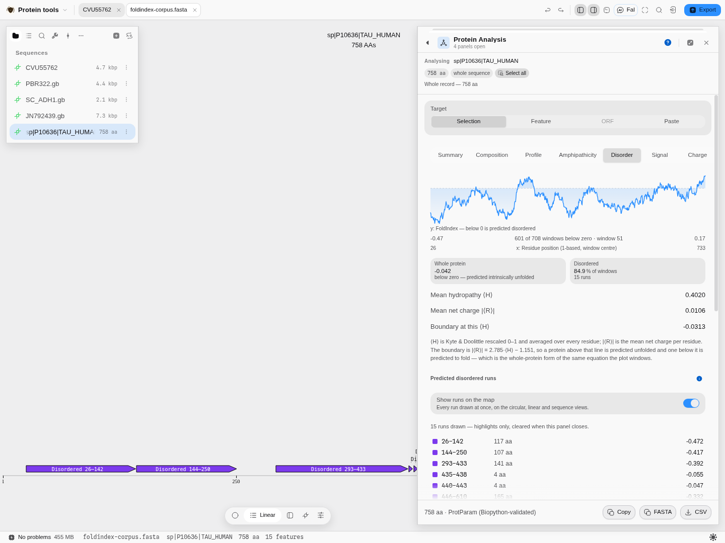 Tau in the Disorder tab: 601 of its 708 windows score below zero, in 15 separate runs, and every one
of them is drawn on the sequence below.
3 · Check the two tiles. Whole protein is the same equation applied to the sequence as a whole rather than to a window, so it is one number you can quote: tau scores −0.042. Disordered is the share of windows below zero and the number of separate runs they form.
3b · Run a rigid protein too, so you know what the other end looks like. The sample project also
carries bacteriorhodopsin (P02945), a seven-helix membrane bundle with no disordered region at all:
0 of its 212 windows fall below zero and the whole-protein score is +0.438. Reading that
beside tau is what calibrates the scale — a method that only ever ran on disordered proteins would
look equally confident on both.
4 · Read the three rows underneath, because they are the actual coordinates. Mean hydropathy ⟨H⟩ and mean net charge |⟨R⟩| are where this protein sits on the charge–hydropathy plane, and Boundary at this ⟨H⟩ is the line it is being judged against. A protein above its boundary is predicted unfolded; below it, predicted to fold. Two proteins can share a FoldIndex score for opposite reasons — one low in hydropathy, one high in charge — and only these rows tell them apart.
5 · Draw the runs on the map. Switch on Show runs on the map and each stretch of consecutive below-zero windows appears as a violet span on the circular, linear and sequence views. That is the question the plot cannot answer: which part of my construct is predicted disordered. Hovering a span gives the residue range, the mean and deepest score in it, and the window that produced it. A span marks window centres — each window reads half its width further either side, so the real region is a little wider than the mark, and the tooltip says so rather than guessing a boundary.
6 · Click into it. Clicking a point on the curve selects the residues that window covered; clicking a run in the list selects the run. From there the selection is a target for every other tool — send it to Protease digest to see which peptides a disordered tail would give, or to Back-translate to order a construct without it.
7 · Change the window and watch what happens. 51 residues is the size the method was published with. Narrow it to 21 and short dips appear that the wider window smoothed away; widen it to 101 and only domain-scale answers survive. There is no correct value — the window is the question you are asking, which is why it is a control and not a constant.
8 · Now run the two proteins it gets wrong. This is the most useful five minutes on the page.
The sample opens on tau; to reach the others, open the file's record list — the ⋮ beside
foldindex-corpus.fasta, then File properties → Show 12 records — and click the one you want.
Each opens as its own document, in its own tab, so you can flip between them.
α-synuclein is a textbook natively-unfolded protein and FoldIndex scores it +0.053 — just on the
folded side — because its amphipathic N-terminal repeats are hydrophobic enough to outweigh its
acidic tail. GFP is a rigid β-barrel and 55.9% of its windows come out negative, because its fold
is held by a barrel rather than by a high mean hydrophobicity. Both are in the sample. A composition
average cannot see either case, and knowing that is the difference between using this tool and
trusting it.
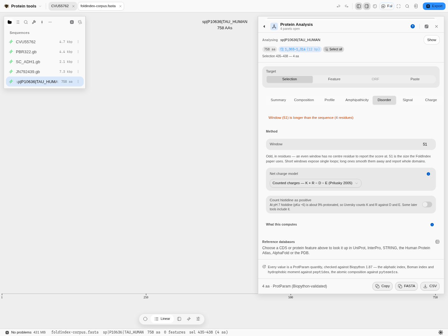 Scope the panel to a four-residue run and a 51-residue window has nothing to sit in. The reason
appears above the control that caused it, rather than leaving you with an empty plot to interpret.
Pro tips and pitfalls
- A negative score is a hypothesis, not a result. Prothymosin α, at 100% of windows below zero with a whole-protein score of −0.765, is about as strong as this signal gets. A protein scoring −0.02 is telling you very little.
- Long, monotonous, low-complexity sequence is what it detects best — and coiled coils, collagen repeats and long linkers can all read as disordered when they are not.
- The window must be odd, because the score is reported at the window's centre residue; the panel refuses an even one instead of quietly shifting the axis.
- It refuses non-standard residues by name. An
Xor aBis not scored as if it were something else — on the rescaled hydropathy scale, zero is arginine, so a placeholder residue would drag every window containing it toward "disordered" without saying so. - Compare within one protein, not between two run at different settings. The window, the charge model and the pKa set all move the number; the panel reports all three next to the result and the CSV carries them on every row.
What it hands to and takes from other tools
The disordered runs are a selection like any other, so they flow outward: to Protease digest, Back-translate, the Codon Optimizer, or the primer designer once the region is back in DNA. It takes its target from wherever you came from — right-click a CDS on the map, or a feature in the rail, and the panel arrives already scoped to it.
The science
Every quantity is a published one and is computed the way its source defines it: mass from the residue masses plus water; the isoelectric point by iterating the charge equation to zero; the instability index from Guruprasad's dipeptide weights; the aliphatic index after Ikai (1980); GRAVY as the mean Kyte–Doolittle value; the extinction coefficient from tryptophan, tyrosine and cystine counts.
The profiles are the ProtScale method: pick a scale, average it over a sliding window, optionally weight the window's edges, optionally normalise the scale first.
Signal-peptide cleavage sites are von Heijne's weight-matrix method: a log-odds score over the 13 residues before the cut and the first two after, with positions −1 and −3 weighted as the later refinement of the method specifies.
Where the numbers are checked. These are the ProtParam quantities and they are verified against
Biopython — the aliphatic index, Boman index and hydrophobic moment against the peptides reference
implementation, the atomic composition against pyteomics. The panel states this at its foot, so the
claim travels with the numbers. The cleavage-site matrices and every score computed from
them are checked against EMBOSS, cell by cell over both matrices — and the worked example above is a
second, independent check: the prediction reproduces the cleavage site pBR322's own curated record
annotates.
Limitations
- A predicted property is not a measured one. The instability index in particular is a sequence-derived correlate of half-life in E. coli, not a measurement of your protein in your cells.
- The extinction coefficient assumes folded, native tryptophans. It is the standard assumption and it is wrong for a denatured or heavily modified protein.
- ProtScale's exponential weight model is reproduced, not quoted. ExPASy never published its formula. The one used here was recovered from ProtScale's own output and is checked against that service's scores at every window it offers, to the three decimals it prints; a future change to the service would show up as a disagreement there first.
- Non-standard residues leave some values undefined, and the panel says so instead of substituting a standard residue's mass.
- Windowed profiles are blind at the ends. A window of 9 has no value for the first and last 4 residues; the curve starts and stops accordingly rather than being padded to the full length.
- The runs are a classification of windows, not a structure prediction. A transmembrane run here is a hydrophobic-moment signature, not a topology model.
- The signal-peptide scan locates a cut; it does not classify a protein as secreted. A high score says a sequence looks like a cleavage site, not that the protein is exported. Whether it is actually secreted is a separate prediction, and the Topology tab answers a different question again — where the membrane-spanning segments are and which side each terminus sits on.
- Both trained predictions here are single models, and neither is the last word. Membrane topology is HMM-TM and disorder is metapredict or FoldIndex; each is one method, and each has documented cases it gets wrong. Both tabs name an independent predictor at EMBL-EBI and hand off to it — Phobius and TMHMM for topology, MobiDB-Lite for disorder — which is worth taking whenever the confidence is low, the score sits near the boundary, or the call decides a construct.
On disorder specifically
metapredict learned to reproduce other predictors' consensus, so it inherits their blind spots as well as their strengths, and its scores are a prediction of disorder, not a measurement. Signal peptides and transmembrane segments are not what it was trained to call, and an N-terminal signal peptide often scores as disordered. Where it and FoldIndex disagree on the whole protein, the reading says so; that is the case worth an independent check.
FoldIndex reads composition through a sliding window and nothing else — no evolutionary information, no structure, no trained model. That is its virtue (it is instant, local and fully explainable) and its ceiling. It will miss a disordered region that happens to be hydrophobic, and it will over-call a fold that is held by geometry rather than by a hydrophobic core. Where the answer matters, treat it as the screen that tells you which regions are worth a slower method.
Its failures run in both directions, which is why the tab says so rather than leaving you to find out. α-synuclein — a textbook natively-unfolded protein — scores +0.053 and is called folded by a whisker, while a compact fold held by geometry rather than by a hydrophobic core can be called disordered. Within ±0.1 of zero the panel therefore prints a caution naming this run's own score, and offers the MobiDB-Lite check beside it. Treat any score in that band as undecided.
Compared with other tools
No rows yet. Every comparison on this site carries a first-party, dated source, and the competitor material on file says nothing about protein physicochemical analysis. An unsourced row is worse than an absent section.
Export
Copy puts the residues on the clipboard, FASTA writes them as a record, and CSV exports the values.
The composition chart takes a second form when you open it on the canvas: alongside the picture it offers the composition as its own table — one row per amino acid with its count and its percentage of the chain, and, tagged as a second kind in the same file, one row per element of the molecular formula with its share of the atom count. Every one of the twenty amino acids gets a row whether or not the protein contains it, so a zero is a stated absence rather than a missing line: that is the half a bar chart hides worst, and no cysteine and no tryptophan are two of the things a bench reader most often wants off a composition. Percentages are of total length, so a sequence carrying non-standard residues sums to under 100, which is what ProtParam reports too. The panel also hands its exact region to Optimize codons, Codon usage, Protein Domains, Protease Digest, Back-translate and Design primers, so the next tool starts on the same residues without a second selection, and it can save the translation into the project as its own protein record.
The Composition and Charge tabs additionally offer reference-database lookups for the protein by name — UniProt, InterPro, STRING, the Human Protein Atlas, AlphaFold and the PDB. They answer in place, three fields per hit, seeded from the coding feature you already chose so you never retype it; Open in Databases hands the same query to the full panel when three fields are not enough. Nothing guesses an accession for you: the query is the feature's own name, and if you have not chosen a feature the section says so instead of offering a dead button.
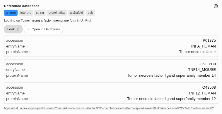 The membrane form of tumour necrosis factor, looked up in UniProt from the feature already
selected. Three hits, each with its accession, entry name and protein name — the human entry and the
two ligand-superfamily members that share the name, which is the distinction you want to see before
you take one.
API
The properties are available headlessly, so the same values can be produced without the panel — the summary quantities, the windowed profiles and the hydrophobic-moment classification are each callable on their own. The editor's Python and R consoles also see the open record, so a calculation of your own can run against exactly what is on screen.
Automation
Available as a workflow node, so protein properties can sit in a DAG — fan it out over several constructs and feed the numbers into the next step.
Provenance
A run records the region analysed, the strand, the genetic code used to translate it, and the conventions in force (the cysteine treatment for ε₂₈₀, the scale, window and weighting for a profile). Citing the method means naming ProtParam and the individual scales, which the panel shows beside each number.
Screenshots
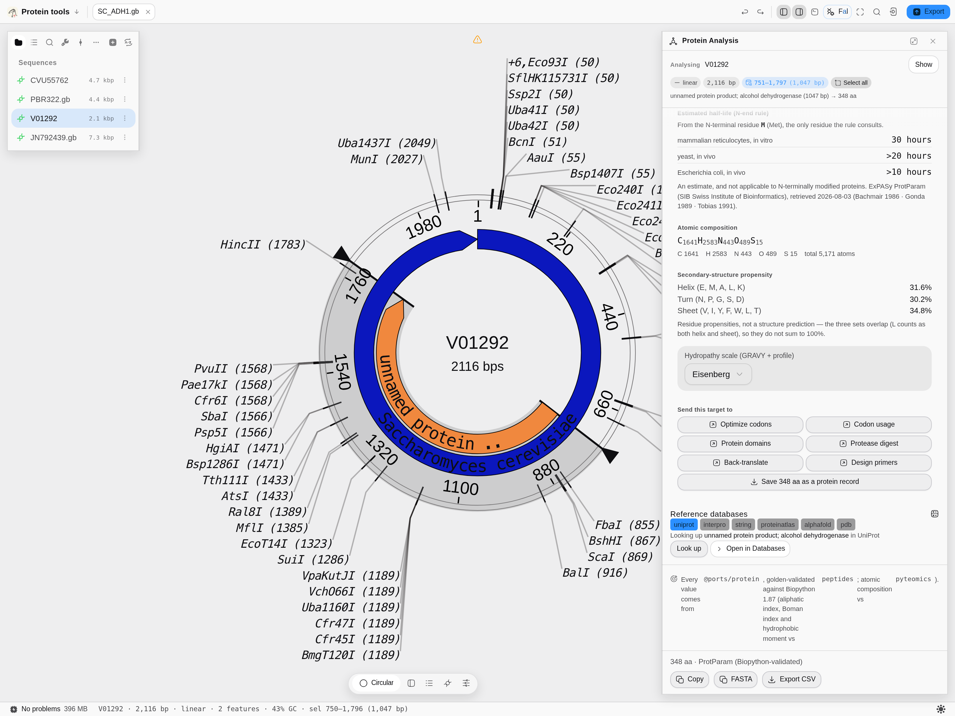 The panel as it opens.
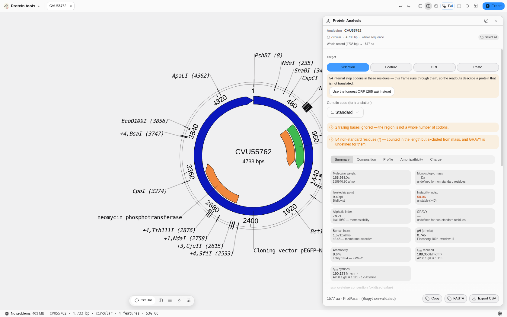 After a run, with real results on screen.
The Disorder tab on tau — the FoldIndex curve, the charge–hydropathy coordinates, and 15 predicted
disordered runs marked on the sequence.
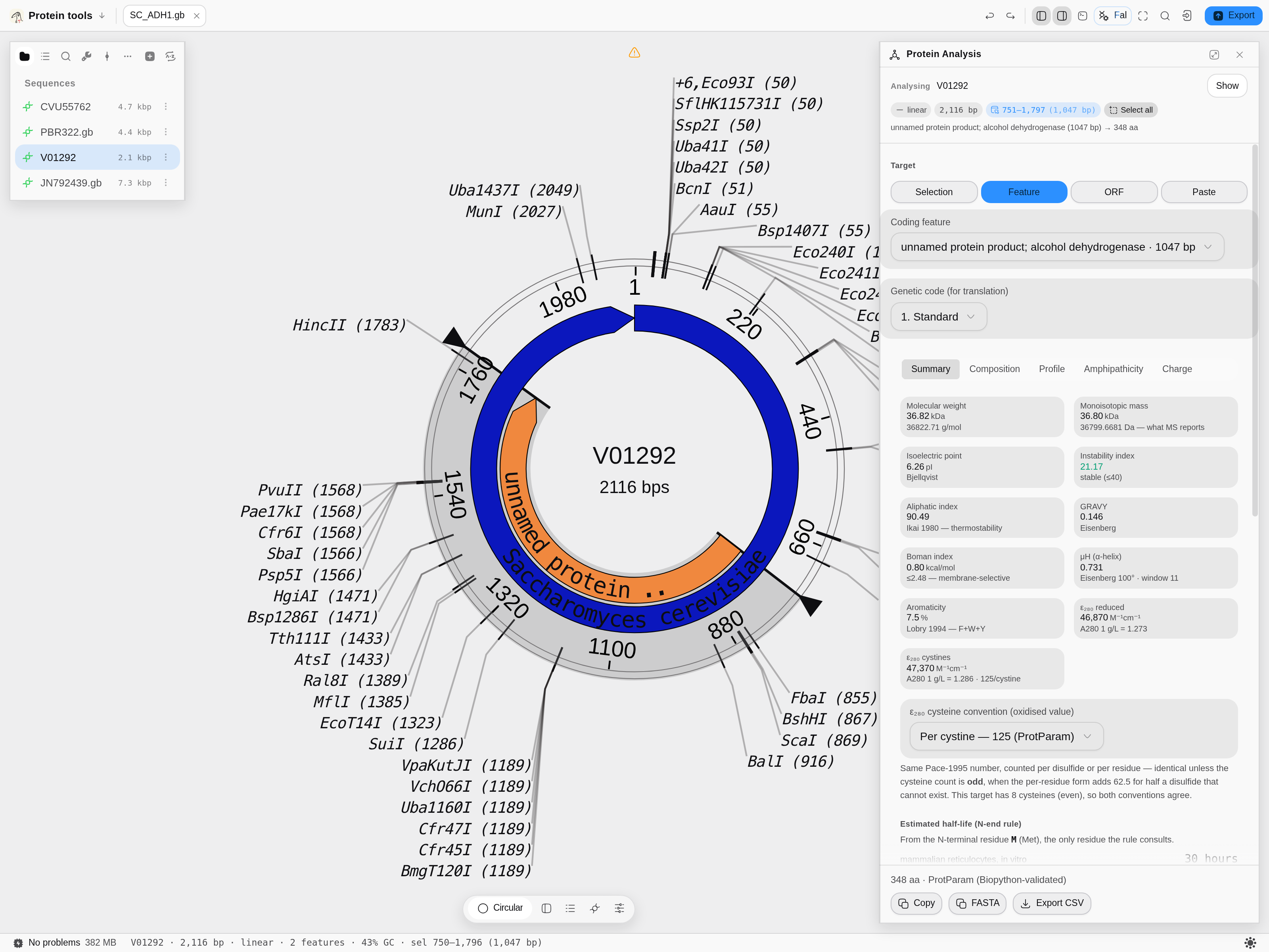 Scrolled, showing the controls below the fold.
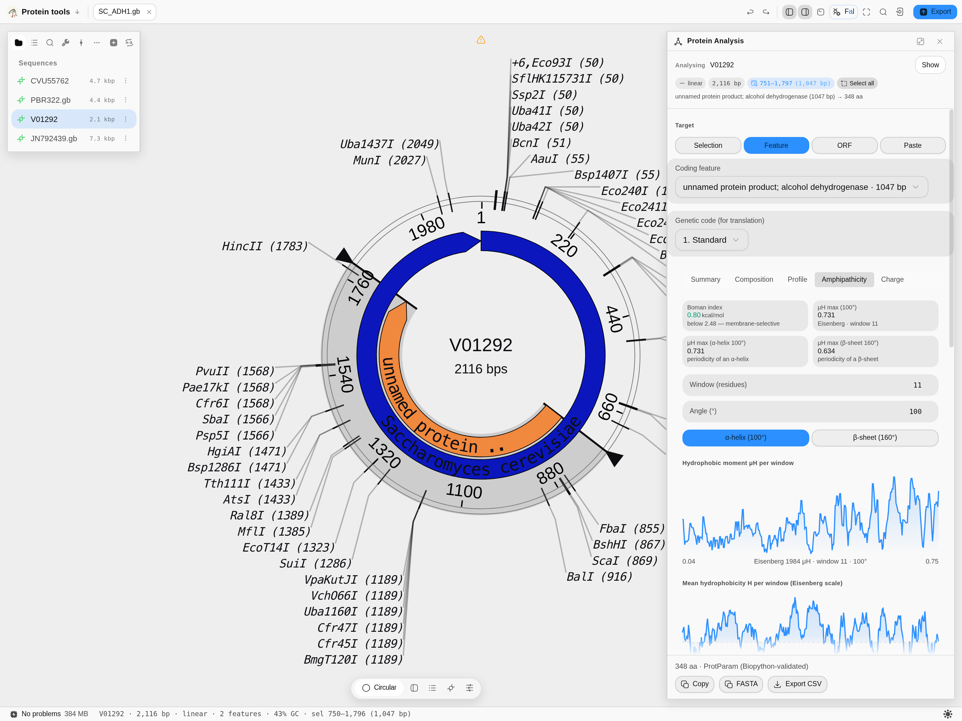 The amphipathicity tab.
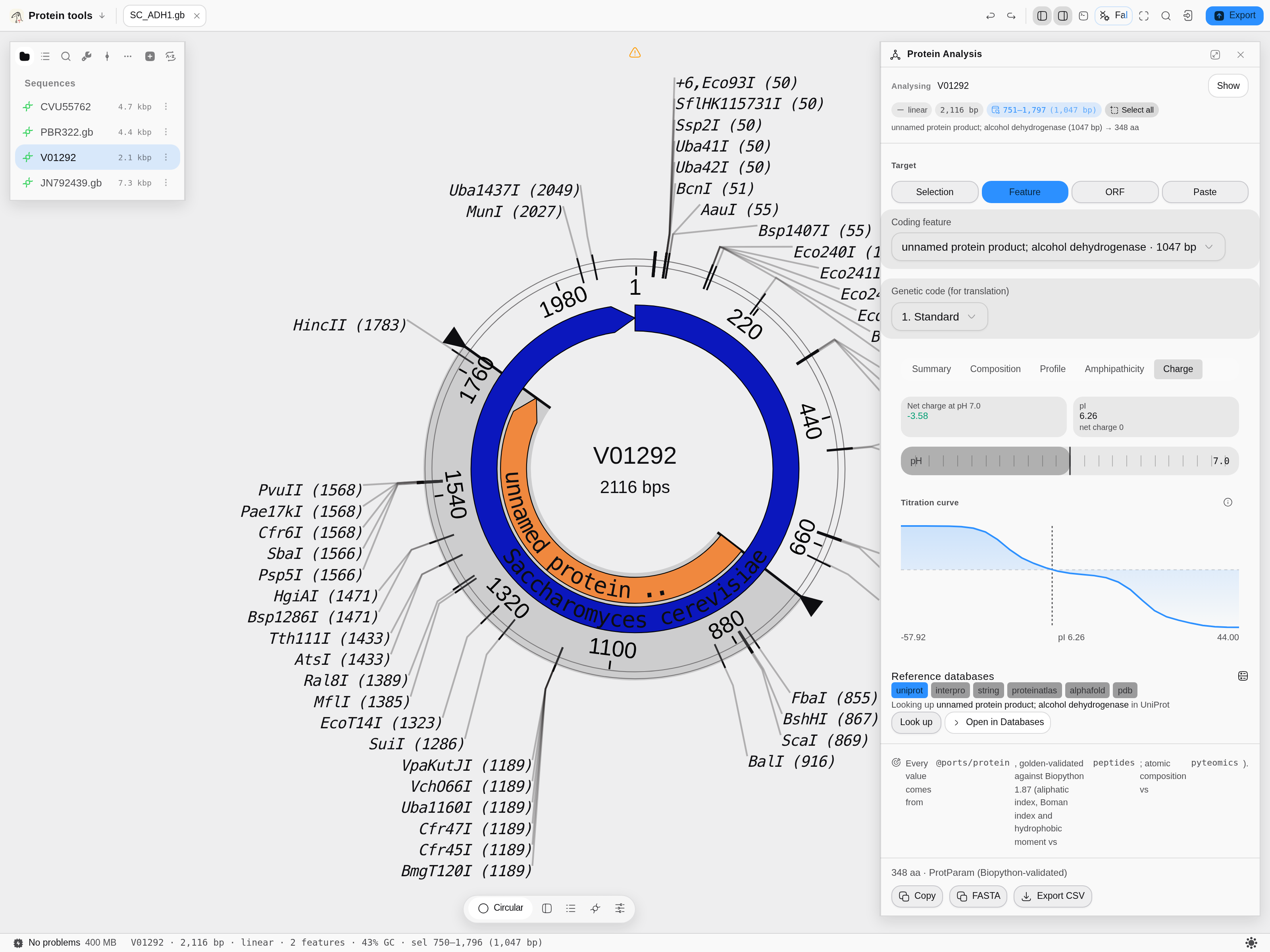 The charge tab.
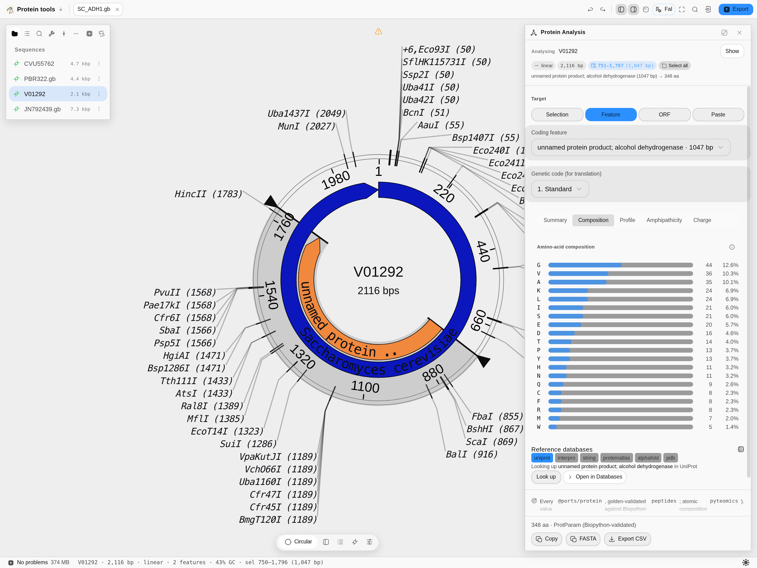 The composition tab.
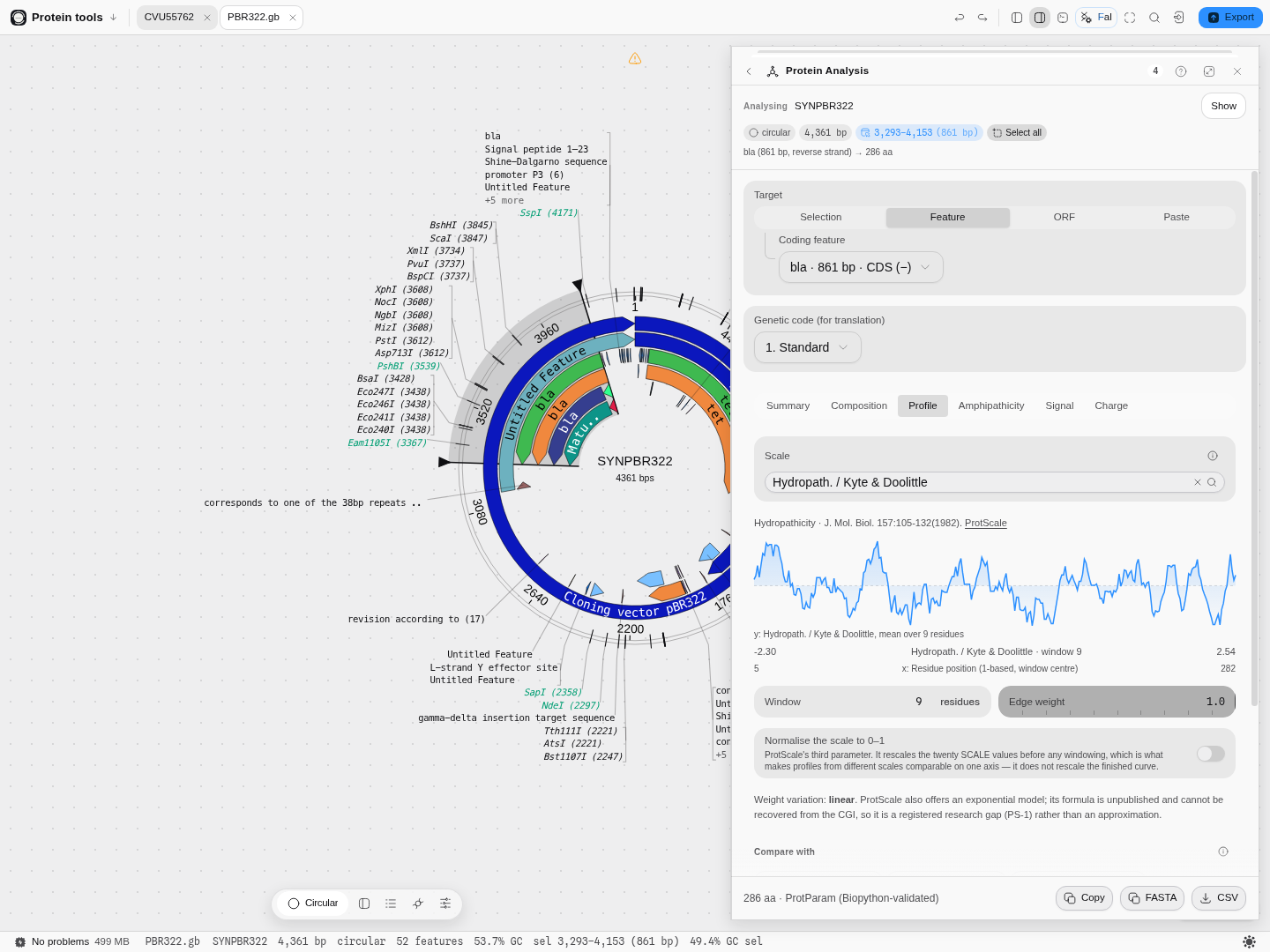 The profile tab.
Related
In this group: Properties · BLAST Search · Search Databases · EMBL-EBI Services · Protein Domains · Protease Digest · Antibody Numbering · Mass spectrometry: peptide masses, b ladders, isotopes, spectrum scoring, q-values, protein inference · Codon Usage Analysis · Site avoidance: restriction sites a genome avoids or favors · Codon outliers: genes whose codon usage departs from their own genome · Tree incongruence: genes whose own alignment rejects the species tree · Reference stability: reference genes against genes of their own abundance · Annotation contradictions: UniProt features a predictor scores unlike confirmed ones · Hypothesis ledger: pre-register a hypothesis, attach runs, decide with e-BH · Reagent audit: does each annotated CDS code for what the map says, and are its cryptic promoters, splice sites and repeats worse than chance · Assay decay: does a published assay still match current genomes, and is the mismatch at the 3′ end · Gene incongruence: which loci of a multi-locus alignment have a different history · Target validation: test "gene G drives phenotype P" against gene-level evidence tables · Codon Tables · Enzyme Collections · Virtual Gel Bench · Phylogenetics · Dot Plot · Table · NumPy Array · Structure · PDF · Molecule · Image
Protein Domains
Take a CDS from the construct you have open, scan it against the InterPro member databases, and put the domains back on the map at DNA coordinates.
Protease Digest
Cut a protein with any of forty-nine proteases and chemicals and read the peptides it would produce, with their masses and m/z, without leaving the construct they came from.