
Codon Usage Analysis
Marked experimental: the surface can change.
Read the codon composition of a coding sequence against a host: which codons are rare in that host, what the codon adaptation index comes to, and how the start and stop context looks.
| Reached by | Tools → Codon Usage Analysis |
| Sample project | Codon usage |
What it does
A gene can encode exactly the right protein and still express badly, because the synonymous choices matter: most amino acids have several codons, and a cell reads some of them faster and more accurately than others. This panel scores a coding region against a reference host and tells you which measure says what, and where along the gene the trouble is.
You give it a coding region and a reference — an organism's codon usage table, or a tRNA gene pool — and it reports the adaptation of the region as a whole, then marks the individual codons and stretches responsible directly on the map.
When you'd use this
Used in: Optimize a coding sequence for expression in another host
Three questions bring people here.
- "Will this gene express in my host?" You have a CDS from one organism and you intend to express it in another. Score it against the host's table: CAI, Fop and the rare-codon list tell you how far it is from what the host prefers, and the map shows you whether the awkward codons are scattered (usually tolerable) or clustered (often not).
- "Where should I change it?" A single number cannot answer that. The %MinMax profile finds the slow stretches, the rare-codon clusters mark translational-pause candidates, and every readout clicks through to the exact bases — so you can hand a specific region to Optimize instead of rewriting the whole gene.
- "Is this gene highly expressed in its own genome?" Score it against its own organism. A high CAI and a high Fop in the native host is the classic signature of a highly-expressed gene.
The usual route is Codon Usage Analysis → Optimize → back here to confirm, with Codon Tables if you need to build or import a reference table first.
What this computes
Nine measures of codon bias, and they disagree on purpose — each asks a different question, none stands in for another, and every number on screen names which produced it.
| Readout | The question | What it needs |
|---|---|---|
| CAI (Sharp & Li 1987) | How close is each codon to its family's most-used codon in the host? | a usage table |
| Fop (Ikemura 1981) | What fraction of codons are among the host's best? | a usage table or a tRNA pool |
| ENC (Wright 1990) | How many codons does this gene effectively use, 20–61? | nothing but the sequence |
| RCBS / DCBS (Roymondal 2009; Sabi & Tuller 2014) | How far is usage from what this gene's own base composition predicts? | nothing but the sequence |
| tAI (dos Reis 2004) | How well does the host's tRNA pool decode these codons? | tRNA gene copy numbers |
| nTE (Pechmann & Frydman 2013) | How well are they decoded given what the rest of the cell is already using? | tRNA copies and transcript abundances |
| CPB (Coleman 2008) | Are adjacent codon pairs under-represented? | reference sequences |
| %MinMax (Clarke & Clark 2008) | Where along the gene is usage extreme? | a frequency table |
| CUFS (Diament, Pinter & Tuller 2014) | How differently do two genes choose codons? | nothing but a second sequence |
The one measure with no host in it. Every row above except ENC, RCBS and CUFS compares a gene against an organism — its published usage, its tRNAs, what its cell is already translating. CUFS compares two genes with each other, so it keeps answering when nobody has published a table for your organism, and it answers the question a construct raises rather than the question a genome does: does the gene you inserted use codons like the rest of this plasmid, or does it stand out? The panel ranks every other coding feature in the record, nearest usage first.
It is a true distance — symmetric, zero only when two genes' codon distributions are identical, and obeying the triangle inequality, which is what lets a set of them be clustered. By default the amino-acid composition is divided out (synCUFS), because without that two genes coding different proteins are far apart mostly for coding different proteins, which is true and is not what anyone means by codon usage. Both forms are offered and the panel says which one produced the number. A gene too short for the statistic is listed as not compared, with its length, rather than left out.
A region that is not a coding sequence is named as one. Codon bias is defined over codons, and a span you chose by eye may not begin at a start codon or end at a stop — an internal exon, a domain, a deliberately chosen window. Where the reference publishes start- and stop-codon usage, the reading says which of the two ends is missing and shows the region's first and last codon, because the same signature is what a whole gene read on the wrong strand or out of frame produces. It is a statement, not a refusal: the scores are still computed and still meaningful for the region you asked about.
Every reading belongs to the region named above it. Each measure here is a statement about one stretch of one molecule, so the panel shows a result only while you are still looking at the coding region it was computed on. Open a different sequence, or move the selection you analysed, and the readings are cleared rather than re-labelled: a codon adaptation index means nothing without knowing which codons it counted, and a number carried under the wrong heading is worse than no number. Press Analyze again and the panel recomputes for what is in front of you.
Per codon and per stretch, not only per gene. The individual codons and the runs responsible for a poor score are marked on the map, which is the difference between "this gene is 0.71" and "these eleven codons are why".
The distinctions the panel keeps straight, because they are the ones people conflate
- CAI measures degree, Fop measures membership. A codon at 79% of its family's peak scores nearly as well as the peak under CAI; under Fop it either clears your threshold or it does not. Fop is therefore the more comparable measure across genes of different amino-acid composition, and the more brutal one
- Fop has two bases and they disagree on real genomes — optimal by frequency in the host's genes, or by the abundance of the tRNAs that read them. Both ship as a switch: the usage table asks what the host prefers, the tRNA pool what it can decode fastest. Choosing an expression host, the second is usually the question you mean
- A measure whose inputs you have not supplied is not estimated. tAI needs tRNA gene copy numbers, nTE needs those and measured transcript abundances; without them the row says so rather than filling in a plausible number
The reference is a control, not a hidden default — which organism's table, or which tRNA pool, and any table you counted yourself in Codon Tables appears here as an ordinary host.
Where it lives
Tools → Codon Usage Analysis, the command palette, or right-click a CDS on the map. Opening it from a feature scopes it to that feature; changing the target selects those bases on the canvas, and every result row and plot position clicks back to the sequence.
Inputs and outputs
In: any loaded nucleotide record — a whole sequence, the current selection, or a CDS/feature you pick. The region must be a whole number of codons; if it is not, the panel says so and offers to trim or extend to the nearest reading frame rather than silently analysing the wrong frame.
A minus-strand feature is read on its coding strand automatically. So is a selection you made by right-clicking a feature — the strand you clicked travels with the span. A selection you drew by hand carries no strand of its own, and for that the read the − strand switch is the answer.
Out: the scores below, a 61-codon usage matrix, every rare-codon and non-optimal position, the along-the-gene profile, map tracks for each of those, and one CSV carrying all of it with a provenance header naming the region, the source, the organism and every setting.
Demo
No screencast yet. The Codon usage sample project below is the demo: it opens on a real gene with the panel already scoped to it, so the worked example can be reproduced click for click.
Worked example
The Codon usage sample project opens on Saccharomyces cerevisiae ADH1 (GenBank V01292), the canonical highly-expressed yeast gene. Target the CDS at 751–1,797 (1,047 bp, 349 codons), choose the bundled CUTG S. cerevisiae table, and Analyze:
| Readout | Value |
|---|---|
| CAI | 0.817 |
| GC | 48.4 % |
| ENC | 31.33 |
| Fop (w ≥ 0.80, usage table) | 0.580 — 202 of 348 scored codons optimal |
| RCBS (geometric) | 0.9071 |
| Rare codons (w < 0.30) | 0 |
Zero rare codons and a high CAI is exactly what a hyper-optimised gene looks like in its own host.
ENC of 31 against a maximum of 61 says the same thing from the opposite direction: the gene uses far
fewer codons than it could. For contrast, run the same project's HC_Amp_ccdB.gb cassette against
the same yeast table — a deliberately rare-codon-loaded sequence — and CAI falls to 0.390 with 42 %
of its codons rare.
Controls
| Control | What it changes |
|---|---|
| Coding region | Whole sequence, current selection, or a CDS/feature. Out-of-frame regions offer a trim/extend rather than a dead button. |
| Read the − strand | Analyses the reverse complement of a selection. A feature brings its own strand and overrides this. |
| Reference source | NCBI RefSeq (live, any organism), CUTG (offline, bundled or the full 35,799-organism release), Kazusa, or the curated pydna tables. |
| Counting basis | Highly-expressed genes (the CAI reference set) or whole genome. |
| Coverage | Every CDS in the assembly, or the largest replicons up to a budget. The readout always states which was actually counted. |
| Rare-codon cutoff | Relative adaptiveness below which a codon counts as rare. Default 0.30. |
| Profile metric / window / cluster cutoff | %MinMax or windowed CAI, the sliding-window width, and the depth at which consecutive windows count as a cluster. |
| ENC background correction | Novembre's (2002) correction of ENC for the gene's GC background. |
| ENC over codon pairs | Alexaki's (2019) extension: the same estimator over codon pairs instead of single codons, kept on the 20–61 scale. Off by default, since single-codon ENC is the value papers report. |
| Fop basis and threshold | Whether "optimal" is defined by the usage table or by the tRNA pool, and the within-family ratio at which a codon qualifies. |
| RCBS directional / reduction | The directional (DCBS) variant, and the geometric or arithmetic mean. |
| Organism | Which organism's reference table is used, with the ones carrying a published CAI reference set marked. |
| Counted CDS | For a live NCBI table, whether highly-expressed genes or every CDS is counted. |
| Optimal at | Ikemura's cutoff for Fop: a codon counts as optimal at this share of its synonymous family's most-used codon. 0.80 is the convention every published Fop uses. |
| ENC over codon pairs (Alexaki 2019) | Scores the effective number of codons over codon pairs instead of single codons, taken to the power 1/k so it stays on the 20–61 scale. |
| Directional (DCBS) | The directional variant of RCBS. |
| Prokaryote · I34 (lysidine) coupling | Adds the prokaryotic lysidine modification to the tAI weights. |
| Abundance set / Assay group / Transcript set | For nTE: which published expression set, which condition within it, and which transcript set the identifiers are matched against. |
| Or use your own abundance table | Two columns per line, a gene identifier then a value, tab- or comma-separated. Any unit works, since demand is scaled to its own maximum. |
| Show on map | One switch per layer: rare codons, clusters, pair junctions, low-tAI codons, non-optimal codons, most-deviant codons. |
| Save to project tables | Keeps the reference table this run scored against, under a name, so other tools can be pointed at the same measurement. Saving the same table twice adds nothing; two different measurements of one organism keep two names, because an E. coli table counted from CUTG and one from Kazusa are not the same table. |
Algorithms you can choose
Codon bias is not one measurement, and the measures disagree on purpose — each asks a different question. All of them ship, none stands in for another, and the panel names which produced each number.
| Measure | The question it answers | Needs |
|---|---|---|
| CAI (Sharp & Li 1987) | How close is each codon to its family's most-used codon in the host? | A usage table |
| Fop (Ikemura 1981) | What fraction of codons are among the host's best? | A usage table or a tRNA pool |
| ENC (Wright 1990) | How many codons does this gene effectively use, 20–61? | Nothing — the sequence alone |
| RCBS / DCBS (Roymondal 2009; Sabi & Tuller 2014) | How far is codon use from what this gene's own base composition predicts? | Nothing — the sequence alone |
| tAI (dos Reis 2004) | How well does the host's tRNA pool decode these codons? | tRNA gene copy numbers |
| nTE (Pechmann & Frydman 2013) | How well are they decoded given what the rest of the cell is already using? | tRNA copy numbers and measured transcript abundances |
| CPB (Coleman 2008) | Are adjacent codon pairs under-represented? | Reference sequences |
| %MinMax (Clarke & Clark 2008) | Where along the gene is usage extreme? | A frequency table |
Three distinctions worth keeping straight, because they are the ones people conflate:
- CAI vs Fop. CAI measures degree — a codon at 79 % of its family's peak scores nearly as well as the peak. Fop measures membership — that codon is either optimal or it is not, at a threshold you set. Fop is therefore the more comparable measure across genes with different amino-acid composition, and the more brutal one.
- Fop's two bases. Ikemura defined optimal codons both by frequency in the host's genes and by the abundance of the tRNAs that read them. Both ship as a switch, because on real genomes they disagree — the usage table asks what the host's genes prefer, the tRNA pool asks what the host can decode fastest. If you are choosing an expression host, the second is often the question you actually mean.
- tAI vs nTE. tAI counts supply: does the cell own tRNAs for these codons? It has no notion of competition, so a codon read by an abundant tRNA still scores well even when every other transcript in the cell is queuing for that same tRNA. nTE divides supply by demand — every codon of every transcript, each weighted by that transcript's measured abundance — so a codon scores well only when its decoder is plentiful relative to how heavily the cell is already using it. The two part company exactly where it matters: on glucose, yeast ADH1 scores tAI 0.611 and nTE 0.148, because ADH1 is itself one of the most abundant transcripts in the cell and its favourite codons are the contended ones.
- RCBS needs no reference at all. It compares the gene's codon frequencies against what its own per-position base composition predicts. That makes it the measure to reach for when your organism has no published table — the one case where CAI, Fop, CPB and the profile all go quiet. Note its two reductions have different neutral points: a gene matching its own composition scores 0 geometrically and 1 arithmetically, and the panel labels which is on screen.
The science
Every score is computed by the same engine the published tools use, reproduced algorithm for algorithm and checked against the original implementations.
Relative adaptiveness w = f / f_max within each synonymous family is the quantity underneath
CAI, the rare-codon scan and Fop's table basis alike — one definition, used everywhere, so the three
can never disagree about the same table.
Fop counts the fraction of codons whose within-family ratio reaches the threshold (default 0.80). Codons from a synonymous family the reference never observed are excluded from both halves of the fraction rather than counted as non-optimal — a family with no evidence is not evidence of a bad codon.
RCBS builds the expected codon composition from the sequence's own base frequencies at each of the three codon positions, then compares observed frequency against that product. The directional variant scores a codon as biased when it is far from expectation in either direction.
Significance (z and p) asks a different question from every score above: given the synonymous choices this gene makes elsewhere for the same amino acid, how unusual is the choice here? Positions are grouped by the residue they encode and each is standardised within its group, so the comparison is internal to the gene rather than against any reference. An amino acid the gene always spells the same way has no comparison group, and no value is shown — a zero there would claim "exactly typical" where nothing could be measured.
%MinMax slides an 18-codon window and reports, per position, how far usage sits between the least- and most-used synonymous options. Consecutive windows at or below −10 % are reported as a rare-codon cluster, the depth at which cluster enrichment becomes statistically significant in E. coli (Chartier, Clarke & Clark 2010).
Correctness provenance: the codon-bias measures are verified against the reference implementations of Ikemura's, Wright's, Roymondal's, Coleman's and dos Reis's methods, value for value over whole reference tables and whole sequences rather than spot checks; CAI, rare codons and the start/stop and N-end readouts are verified against pydna; the CUTG readers are verified against EMBOSS across all 35,799 records of the released database; and the restriction and enzyme data the map draws alongside are checked against REBASE.
Shared with other tools: Codon usage compares how every tool that does this chooses its method.
Measuring translational efficiency (nTE), step by step
nTE answers a question none of the other measures can: is this gene's codon choice good given what the rest of the cell is doing? It is the measure to reach for when you are choosing between synonymous designs for a host you have expression data for, or when tAI looks fine and expression still does not. It needs two real inputs — a tRNA pool and a set of transcripts with measured abundances — and it will not run on a guess about either.
Follow along on the Codon usage sample project, which opens yeast ADH1.
- Pick the coding region. Set Coding region to A CDS / feature…, then the ADH1 CDS (1,047 bp). Codon statistics are only meaningful in frame, and a region whose length is not a multiple of three is refused rather than analysed one base out of register.
- Choose the reference host and run. Set Reference source to CUTG, pick Saccharomyces cerevisiae from the bundled tables and press Analyze CDS. CAI comes back 0.817.
- Load the tRNA pool. In tRNA adaptation index, search GtRNAdb for
S288Cand choose Saccharomyces cerevisiae (S288c Apr 2011). It resolves to 41 anticodons across 275 tRNA genes, and tAI reads 0.611. This same pool is nTE's supply half, so nTE and tAI can never disagree about the tRNA data — only about the divisor. - Load the abundance data. In Translational efficiency (nTE), press Load abundance data. Two real EMBL-EBI Expression Atlas experiments are offered, both yeast cell-cycle series: one on glucose (E-MTAB-8626, 9 conditions) and one on ethanol (E-MTAB-8621, 7 conditions).
- Choose the condition — this is a scientific choice, not a default. Demand depends on what the cell is doing. Pick E-MTAB-8626 and condition g1, then a transcript set, then press Measure demand.
- Read what the pairing actually covered. The panel states it before it lets you read a score: 94 transcripts paired · 0 CDS had no abundance row · 7,033 abundance rows had no CDS in this set. That last number is the honest one — the bundled transcript set is a single chromosome, so the demand it states is coarser than a whole transcriptome would give.
- Read the score, then the profile. nTE comes back 0.148, well below tAI's 0.611. That gap is the finding: ADH1's codons are well supplied and heavily contended, because on glucose ADH1 is itself among the most abundant transcripts competing for them. Click any point on the per-codon plot to select those three bases on the map.
- Put the contended codons on the map. Switch on Show most contended codons on map and the worst-scoring codons draw in indigo along the coding region, deliberately a different colour from the sky-blue tAI layer — so with both on you can see a codon that is well decoded and still contended, which is the case nTE exists to find.
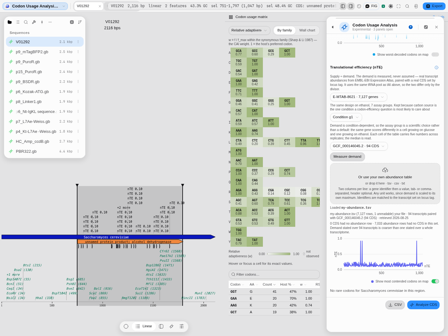
Change one thing and watch it move. Switch the experiment to the ethanol series and re-measure: the same gene scores 0.406. Nothing about the gene or the tRNA pool changed — only what the rest of the cell was doing. If a knob like that does not move your answer, the demand data is not reaching the score, and that is worth knowing before you trust it.
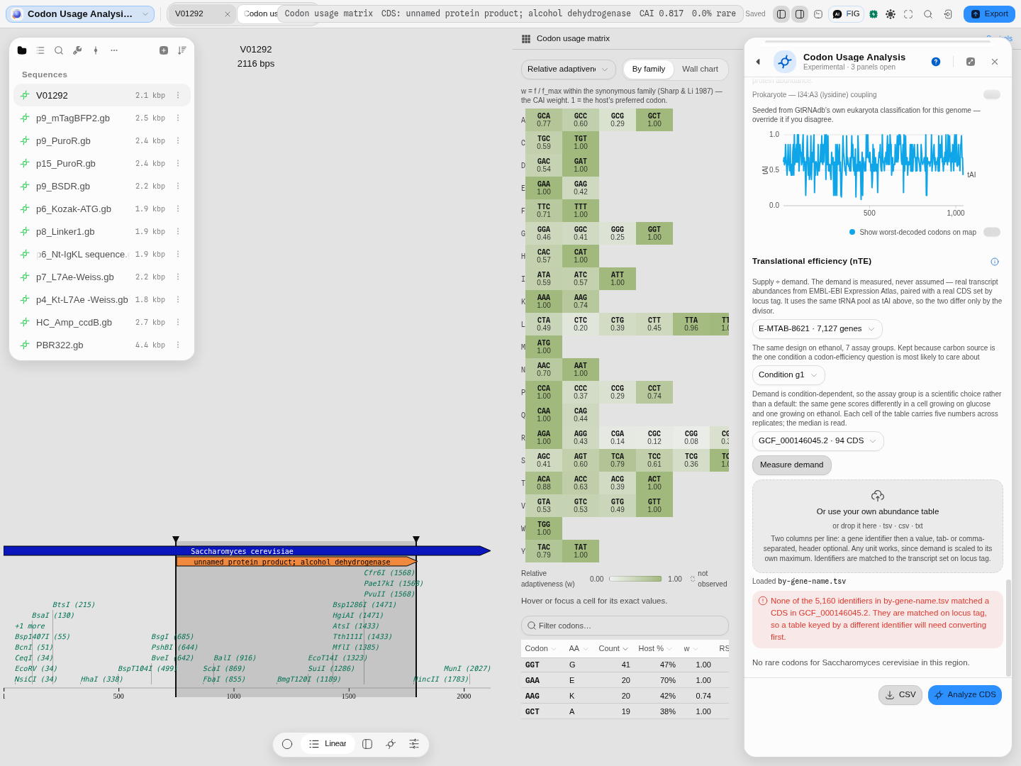
Bringing your own data. The bundled tables exist so the method can be exercised offline; the authority is Expression Atlas, and both files keep their accession so they can be refreshed. To use your own measurements, drop a table into Or use your own abundance table: two columns per line, a gene identifier then a value, tab- or comma-separated, header optional. The unit does not matter — demand is scaled to its own maximum, so only the ratios between transcripts count. The panel reports how many rows it read and how many it could not, and if none of your identifiers match the transcript set it says so and tells you what it matched on, rather than returning a score built from nothing.
Limitations
- Three of the reference sources are fetched live, and a fetch can fail in two different ways. NCBI RefSeq, the Kazusa mirror behind %MinMax and the GtRNAdb genome behind tAI are read over the network when you choose them; only the bundled CUTG and pydna tables work with no connection at all. The panel distinguishes the two failures on purpose, because they call for different things: the service could not be reached (a connection, proxy, firewall or outage — the reading is simply absent, and retrying later is the remedy) versus the service answered and has no table for this organism (a real answer about coverage, which no amount of retrying changes — choose another source, or another assembly). A refusal is reported in the service's own words, naming the genome or organism it was asked about, rather than being restated as a connection problem.
- A table is a summary, and pair statistics are not in it. Codon-pair bias needs the reference sequences, so it is available on the NCBI source and not on Kazusa, CUTG or pydna. The panel says so rather than showing an empty tile.
- The %MinMax profile needs frequencies, not adaptiveness. The pydna tables ship relative adaptiveness, so the profile is not offered there; you can explicitly borrow a Kazusa frequency table for the same organism, and the plot then names the different authority it stands on.
- CUTG is frozen at GenBank release 160 (June 2007). It is bundled and complete for what it covers, but it is a snapshot; its maintained successor is not currently distributable as files.
- ENC is only meaningful over a whole CDS. Over a short region, families that were never observed are imputed as unbiased, which pulls the value up — a poly-alanine sequence scores 46, not 20.
- %MinMax is undefined where there is no synonymous choice. A window of only methionine and tryptophan codons has no range to sit within, and the plot draws a gap rather than a zero, which would read as "average usage".
- A single number cannot tell you a gene is unexpressible. Codon usage is one factor among mRNA structure, GC content, repeats and regulatory context. Use the profile and the map to locate candidates, then test.
- nTE is only as good as the transcript set behind it. The bundled demand set covers one yeast chromosome, 94 transcripts, and the panel says so on screen; that is enough to see the method work and too coarse to publish. Point it at a whole-transcriptome CDS set for a real answer. If a codon is never used by the transcript set you chose, its demand is zero, the arithmetic collapses, and the panel refuses with the offending codons named rather than printing the collapsed score.
- nTE is never approximated from a usage table. Demand is codons weighted by how abundant each transcript is; an unweighted codon count is a different quantity, and substituting one would turn nTE into a rescaled tAI under another name. If there is no abundance data loaded, there is no nTE.
- Significance is a screening statistic, not a permutation test. The z-scores and p-values are the fast analytic estimate rather than a full permutation; z-scores track the permutation result closely, but p-values run lower than a permutation would give — so treat a small p as "look here", not as a published result. They also compare a gene against itself, so they cannot tell you the gene is unusual among genes.
- The scalar scores carry no significance test. CAI, Fop, ENC and RCBS are each a point estimate against a reference, so comparisons between genes of very different length or composition should be read with that in mind.
Compared with other tools
Not yet written. A comparison here would need each incumbent's current behaviour established from its own documentation with a retrieval date, and that has not been done for this tool — so rather than characterise other people's software from memory, this section stays empty on purpose. What can be said without a source is only about this panel: the measures listed above ship together, against the same region and the same reference, with each one's disagreement with the others treated as the point rather than as something to reconcile. That now includes nTE, the only one here that needs measured expression data rather than a table, exposed with its condition as a control rather than a buried default.
Export
CSV, from the panel footer: a provenance header naming region, strand, source, organism and every setting and score, then the 61-codon matrix, the rare-codon locations, the profile and its clusters, the codon-pair junctions, and the per-codon tAI, Fop and RCBS blocks — each with absolute coordinates so a row can be traced back to the base. The codon matrix also opens as its own canvas tab.
API
The codon-usage analysis is available to the in-app Python and R consoles and to the workflow builder, so a score can be computed without opening the panel. It takes an in-frame coding sequence and a reference — either one of the curated organisms, or, for any organism at all, a usage table you have kept in the project — and returns the codon-adaptation index, GC, the codon count, the rare-codon fraction, every rare-codon occurrence with its position, and the two reference-free measures: the effective number of codons and the relative codon bias.
Which reference answered is part of the result, because two of the numbers are not comparable across it. A score against a curated organism reports rare codons from that organism's published low-usage list, which no threshold moves; a score against a usage table reports codons whose relative adaptiveness falls below the cutoff you set. Both are legitimate answers to "is this codon rare", and they are answers to different questions, so the result names the table it used and which of the two rules produced the count.
Automation
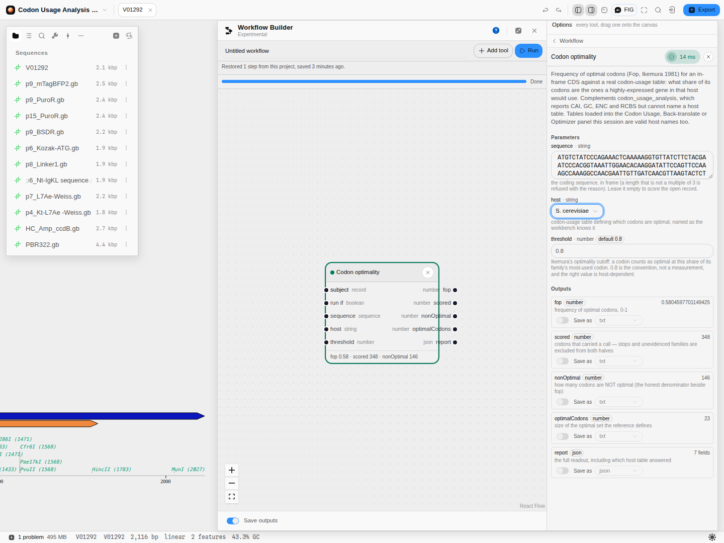
To score many sequences, use the workflow builder rather than repeating the panel: a codon-usage node takes a sequence and a reference organism and emits those values as typed outputs, so a batch over a project's records is a graph. The scientific copilot can run the same analysis and read the numbers back.
Fop is a step of its own. The codon-usage node reports CAI, GC, the rare-codon scan, ENC and
RCBS — everything that is a property of the sequence alone. Frequency of optimal codons needs a
reference table to say what "optimal" means, so it is a separate step, Codon optimality, which
takes a table by name — any bundled host, or any table kept in the project — plus Ikemura's
threshold, and emits fop, how many
codons were scored, how many are not optimal, and how large the optimal set is — and it says whether
the table was a bundled one or the project's own, since two tables can carry one organism's name.
Leave its sequence empty and it scores the open record. A sequence that is not a whole number of codons is refused with
its length, rather than scored on a truncated frame.
Naming the host is the whole point of the step: the same yeast ADH1 CDS scores Fop 0.58 against the S. cerevisiae table and 0.38 against E. coli K-12 — the gene has not changed, the question has.
What automation still does not cover. tAI (a tRNA pool), codon-pair bias (reference sequences) and Fop's tRNA-pool basis each need a reference the automation layer has to fetch rather than look up, so they remain panel-only for now. Batch-scoring those means running them in the panel one region at a time.
Provenance
Each run records the region, the reference source and organism, the counting basis and coverage, and every threshold, so a result can be reproduced exactly. Where a table came from a cache, the readout says whether it was fetched or reused, and how many CDS and codons it was counted from — and whether those counts were published by the file or derived by counting.
An nTE result additionally records which experiment and condition the abundances came from, which transcript set they were paired with, how many transcripts paired, and the retrieval date of the cached copy — all of it in the readout and in the exported CSV, because a supply-over-demand number means nothing without the demand it was measured against. The engine behind it is checked against the published reference implementation of the method, value for value across every codon.
Screenshots
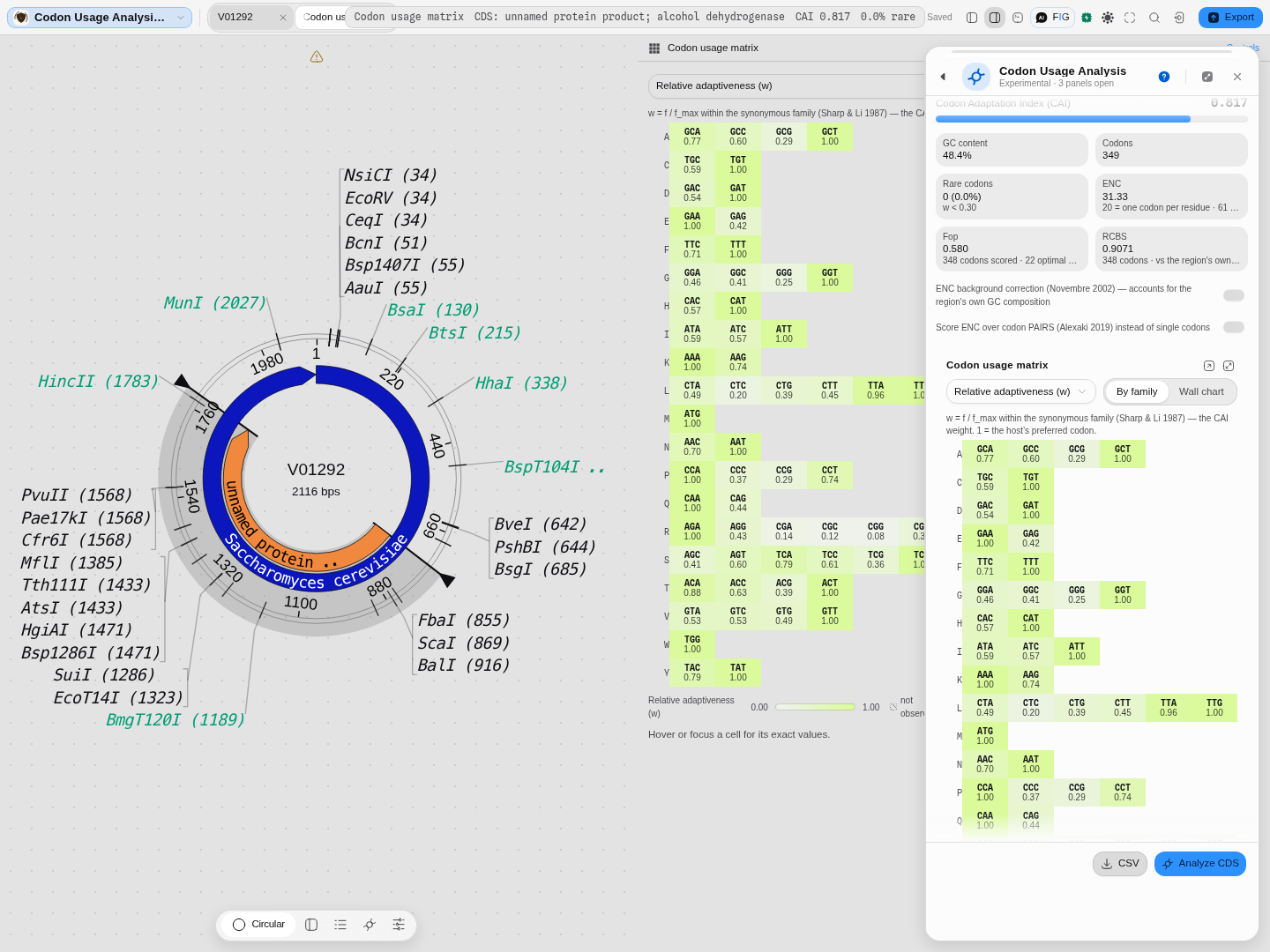 Yeast ADH1's 349 codons scored against E. coli usage — the question you ask before expressing a
yeast gene in a bacterium. Six numbers, not one: CAI 0.817 is the geometric mean of each codon's
relative adaptiveness; ENC 31.33 says how many codons the gene effectively uses out of 61 (20
would be one per residue); Fop is the fraction that are optimal at your chosen threshold;
RCBS measures bias against the region's own base composition, so a GC-skewed gene is not
mistaken for a biased one. The two switches below correct ENC for GC background (Novembre 2002) and
score codon PAIRS instead of single codons (Alexaki 2019).
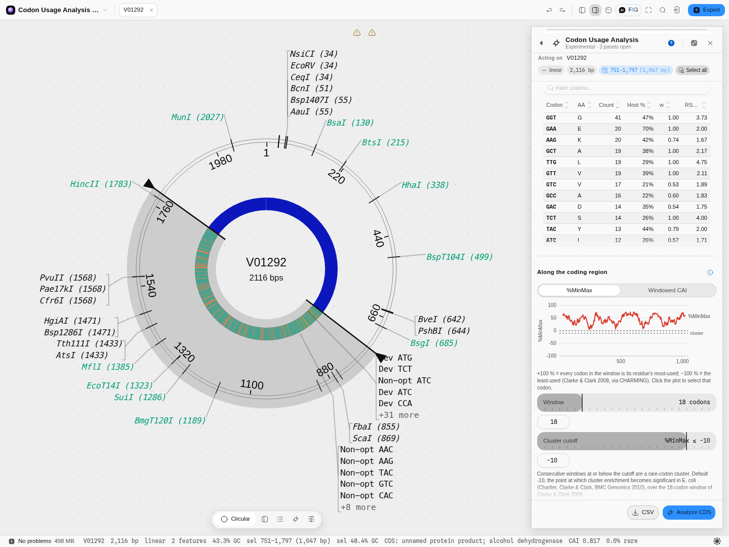 The %MinMax profile along a coding region, with the two controls that shape it. Window sets how
many codons are averaged at each point — wider smooths, narrower resolves single slow patches — and
cluster cutoff sets how far below zero a run has to sit before it counts as a rare-codon cluster.
+100% means every codon in the window is its residue's most-used one; −100% means the least-used.
The gene shown never falls below 0%, which is what a highly-expressed housekeeping gene looks like,
so the cluster list correctly reports none rather than inventing a worst offender.
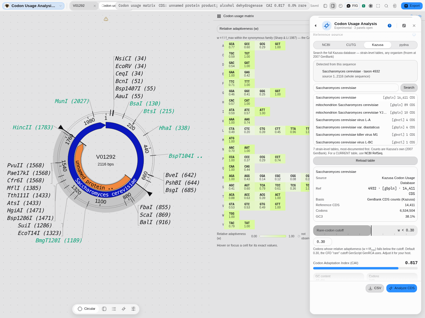 Kazusa searched live, by organism name: seven tables for Saccharomyces cerevisiae alone —
nuclear, mitochondrial, two strains, and three of its viruses — because "the organism's codon usage"
is rarely one table. Picking one states what it stands on: taxon 4932, GenBank division
gbpln,
14,411 CDS, 6,534,504 codons, GC3 38.1%. Kazusa is frozen at the 2007 GenBank release, which the
panel says next to the result rather than in a footnote; for current counts use NCBI RefSeq.
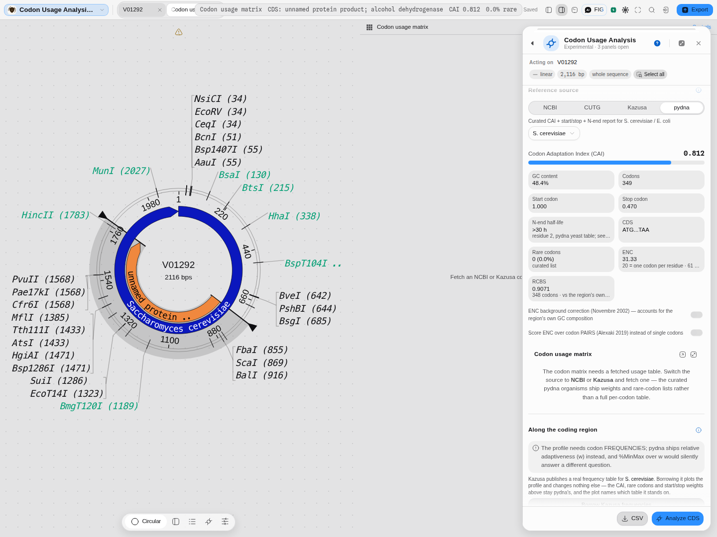 pydna's curated tables answer questions the others cannot: how strong the start and stop
codons are in this host, and the N-end rule half-life implied by residue 2 (>30 h here — a
stabilising residue). It also declines two things rather than approximating them, and says why: it
ships relative adaptiveness rather than frequencies, so there is no per-codon matrix to draw and no
honest %MinMax to compute. That refusal is the point — %MinMax over adaptiveness would return a
number, and the number would answer a different question.
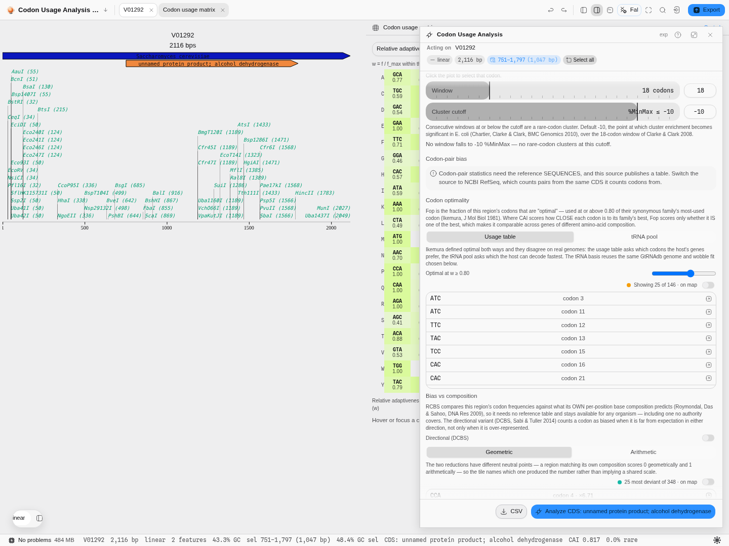 Fop and RCBS on the yeast ADH1 CDS against the bundled CUTG S. cerevisiae table: the basis switch
between the usage table and the tRNA pool, the optimality threshold, the non-optimal codon list with
its real denominator, and the directional and reduction choices for RCBS.
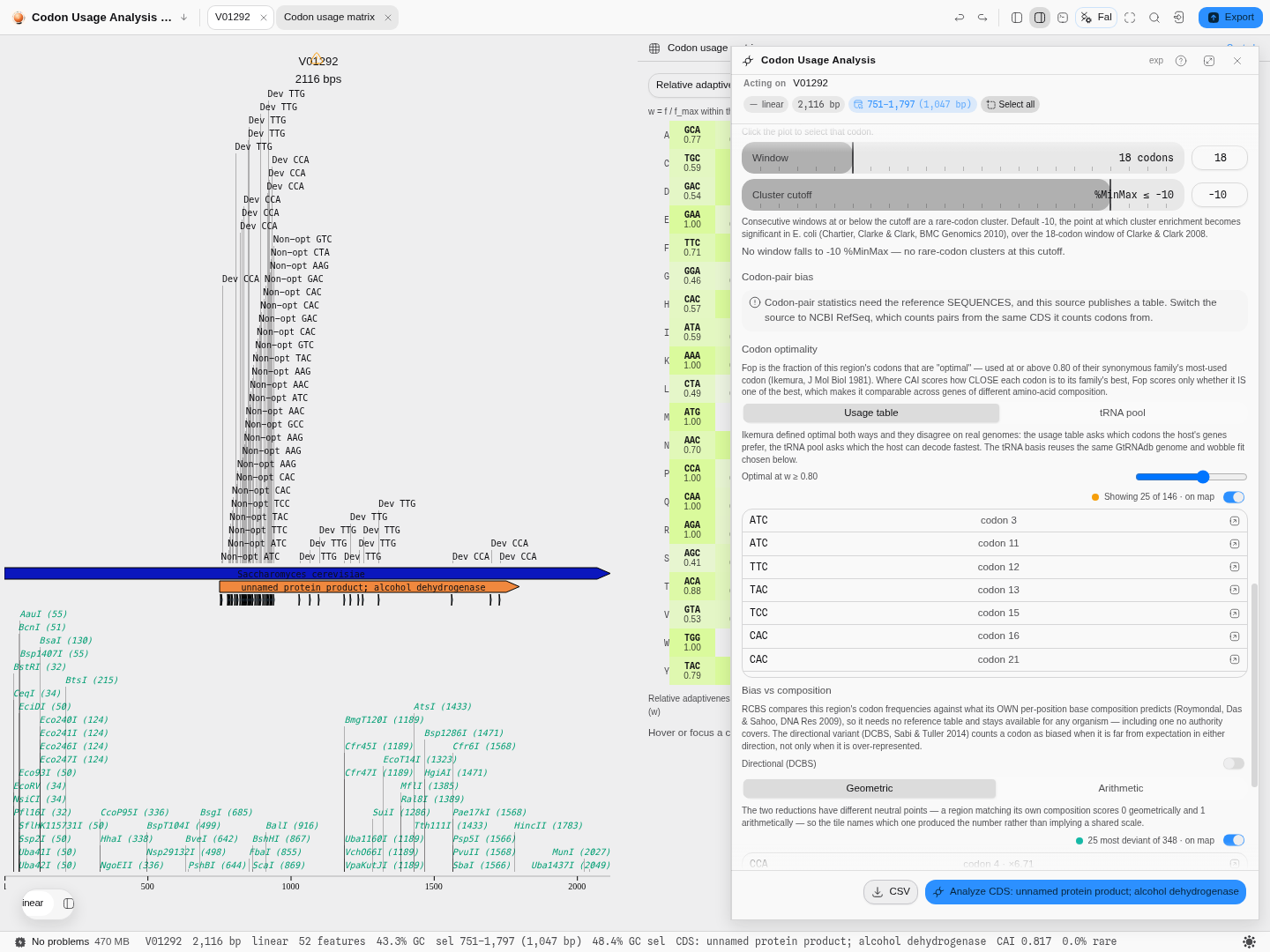 Both measures mark the sequence: amber for codons the reference does not consider optimal, teal for
those furthest from what the gene's own base composition predicts. Every mark carries its value and
citation in the tooltip, and every row in the panel selects the bases.
Related
In this group: Properties · BLAST Search · Search Databases · EMBL-EBI Services · Protein Domains · Protein Analysis · Protease Digest · Antibody Numbering · Mass spectrometry: peptide masses, b ladders, isotopes, spectrum scoring, q-values, protein inference · Site avoidance: restriction sites a genome avoids or favors · Codon outliers: genes whose codon usage departs from their own genome · Tree incongruence: genes whose own alignment rejects the species tree · Reference stability: reference genes against genes of their own abundance · Annotation contradictions: UniProt features a predictor scores unlike confirmed ones · Hypothesis ledger: pre-register a hypothesis, attach runs, decide with e-BH · Reagent audit: does each annotated CDS code for what the map says, and are its cryptic promoters, splice sites and repeats worse than chance · Assay decay: does a published assay still match current genomes, and is the mismatch at the 3′ end · Gene incongruence: which loci of a multi-locus alignment have a different history · Target validation: test "gene G drives phenotype P" against gene-level evidence tables · Codon Tables · Enzyme Collections · Virtual Gel Bench · Phylogenetics · Dot Plot · Table · NumPy Array · Structure · PDF · Molecule · Image
Mass Spectrometry
Weigh a peptide, list the fragment ions it breaks into, score a measured MS/MS spectrum against it, estimate how many identifications are false, and infer which proteins they came from and how likely each is to be present.
Site avoidance: restriction sites a genome avoids or favors
Ask which restriction sites a set of genomes carries far less often, or far more often, than chance predicts.