
Chromatogram viewer
| Document kind | chromatogram |
| Drawn from | a file — it can also be previewed in the file manager |
| Formats that open here | AB1 trace · SCF trace · ZTR trace |
| Refuses to draw below | 280px wide |
What it draws
A Sanger trace: the four dye channels as coloured peaks along the capillary run, with the base the caller assigned to each peak above it, and the per-base quality behind it.
The peaks are the raw evidence. Everything else about a Sanger read — the sequence, the quality, the variant you think you see — is an interpretation of these four curves, which is why this canvas exists rather than a text box holding the called bases.
Four views draw the same read:
- Trace — the peaks alone.
- Split — peaks and base calls side by side.
- Sequence — the base calls as sequence, for when you want to read rather than inspect.
- Reference — the read's peaks drawn under a reference, column by column, which is the view for confirming or dismissing a difference.
Several reads can share one tab, so a forward and a reverse read of the same clone are compared in place rather than in two windows.
What opens in it
AB1, SCF and ZTR traces.
An AB1 carries the most: raw and analysed channel data, per-base quality, the base caller's secondary calls, and the instrument metadata. SCF and ZTR carry the trace and the calls. Anything that depends on secondary base calls — allele phasing in particular — needs an AB1, and says so rather than producing an approximation.
A FASTQ is reads without traces and opens in the read viewer instead; a FASTA of a read that once had a trace has already lost the evidence this canvas is for.
What this computes
The four dye curves are the instrument's; the base calls and qualities are the base caller's, read from the file rather than recomputed. What this canvas computes is everything that turns those curves into something you can judge.
- The trace geometry: each channel's signal placed along the capillary run, with the called base and its per-base quality registered to the peak it belongs to, so a quality value is never read against the wrong position.
- The read's own quality, two ways, because they are different numbers. A Phred score is a log of an error probability, so the arithmetic mean of a read's scores is pulled up by its good bases while its error rate is set by the bad ones: this read's scores average Q19 and the read itself is Q11.1, an expected 92.3% of bases correct. The panel reports the second as read quality with its accuracy, the first as mean of the per-base Phred, and the fraction of bases reaching Q20 and Q30 — definitions on that scale, 1 error in 100 and 1 in 1,000, not chosen cut-offs. It also says how much of the read's whole error budget its sub-Q20 bases carry, which is what decides whether trimming will change the answer. The read-level figure is the one comparable with what long-read and FASTQ tools report as average quality.
- Secondary base calls, where the file carries them — an AB1 does, SCF and ZTR do not. Anything depending on them, allele phasing in particular, requires an AB1 and says so rather than producing an approximation from data that cannot support one.
- Column-by-column correspondence with a reference, in the Reference view: the read's peaks drawn under the reference base they align to, which is the view that confirms or dismisses a difference by putting the evidence under the claim.
- Multi-read registration in one tab, so a forward and a reverse read of the same clone are compared in place — the comparison that separates a real heterozygous site from a one-direction artefact.
- Per-read quality along the run, which is what makes the two ends legible as chemistry rather than as your sample: the first bases run before the separation settles and the last as long fragments stop resolving.
What it does not compute, and will not: whether a double peak is a heterozygote. Two overlapping peaks at one position can be a real heterozygous site, a mixed template, a contaminating colony, or slippage after a homopolymer. The canvas draws the observation and the evidence either side of it; the conclusion is yours.
Reading it
- A double peak is the observation; a heterozygote is a conclusion. Two overlapping peaks at one position can be a real heterozygous site, a mixed template, a contaminating colony, or slippage after a homopolymer. The peak shapes either side, and whether the same position doubles in the reverse read, are what separate them.
- The start and end of every read are bad, and they are bad for reasons of chemistry rather than of your sample: the first bases run before the separation settles, the last as long fragments stop resolving. Judge a read by its middle, and trim before you conclude.
- Quality is the base caller's opinion. It is well calibrated in the middle of a clean read and optimistic across a mixed one.
- A reverse read is drawn as it was run until you reverse-complement it, and the canvas states which orientation you are looking at. Comparing a forward read against an un-flipped reverse read is the classic way to find a difference at every position.
Controls
| Control | What it does |
|---|---|
| View | Trace · Split · Sequence · Reference, as above. |
| Zoom | 2 to 80 px per base. ⌘/Ctrl with the wheel over the trace does the same and keeps the base under the cursor. |
| Peak height | Vertical scale of the peaks, as a fraction of the track height — for reading a weak run without rescaling the whole tab. |
| Trim | The kept range, with the discarded ends shaded on the quality profile. |
| Reverse complement | Flips a track for comparison against a forward read. |
| Base calls | Editable: a call you can see is wrong can be corrected, and the edit travels into every downstream operation. |
The panel beside the canvas carries the rest — the quality profile and mixed-peak count, the vector screen, the alignment and MSA hand-offs, allele phasing, and translation.
Floating a section over the other tabs
Right-click the trace and choose Detach section for any of the three: Quality & peaks, Analyze (align / consensus), or Verify vs reference. The section lifts out of the panel and floats above whichever tab is in front, and this is not just convenience — two of its actions only make sense while you are looking at a different molecule:
- Annotate reference writes the differences into the reference as features, so the reference has to be the tab in front of you. Docked, the section disappears the moment you switch to it.
- quality on map draws this read's Phred scores along the reference (see Graph tracks), and you want to be reading that map while the difference list is still on screen.
The floating card keeps the read's result as you move between tabs, so the sorted difference table and the band drawn on the reference are legible at the same time. That is the whole point: a mismatch sitting in a Q12 trough is a sequencing artefact, and the same mismatch at Q55 is a variant, and no table can tell you which on its own.
Where it appears
As a stage tab when you open a trace, and in the file manager preview, which publishes base count, format, track count and orientation as facts beside the drawing.
Both hosts read the same list of views, so a layout that exists in the editor is reachable in a preview too — a preview has no right-click menu, and a view that lived only there would be a layout the reader simply could not get to.
Performance and limits
- It refuses to draw below 280px wide. A trace is a wide, dense plot; below that the peaks overlap into a solid band, and a clean run and a failed one look the same.
- Long reads at high zoom are wide, deliberately — the canvas scrolls rather than compressing the peaks into an unreadable smear.
- The trace is what the instrument recorded. Nothing here re-calls bases from the raw channels; the calls are the file's, and your edits are yours.
Screenshots
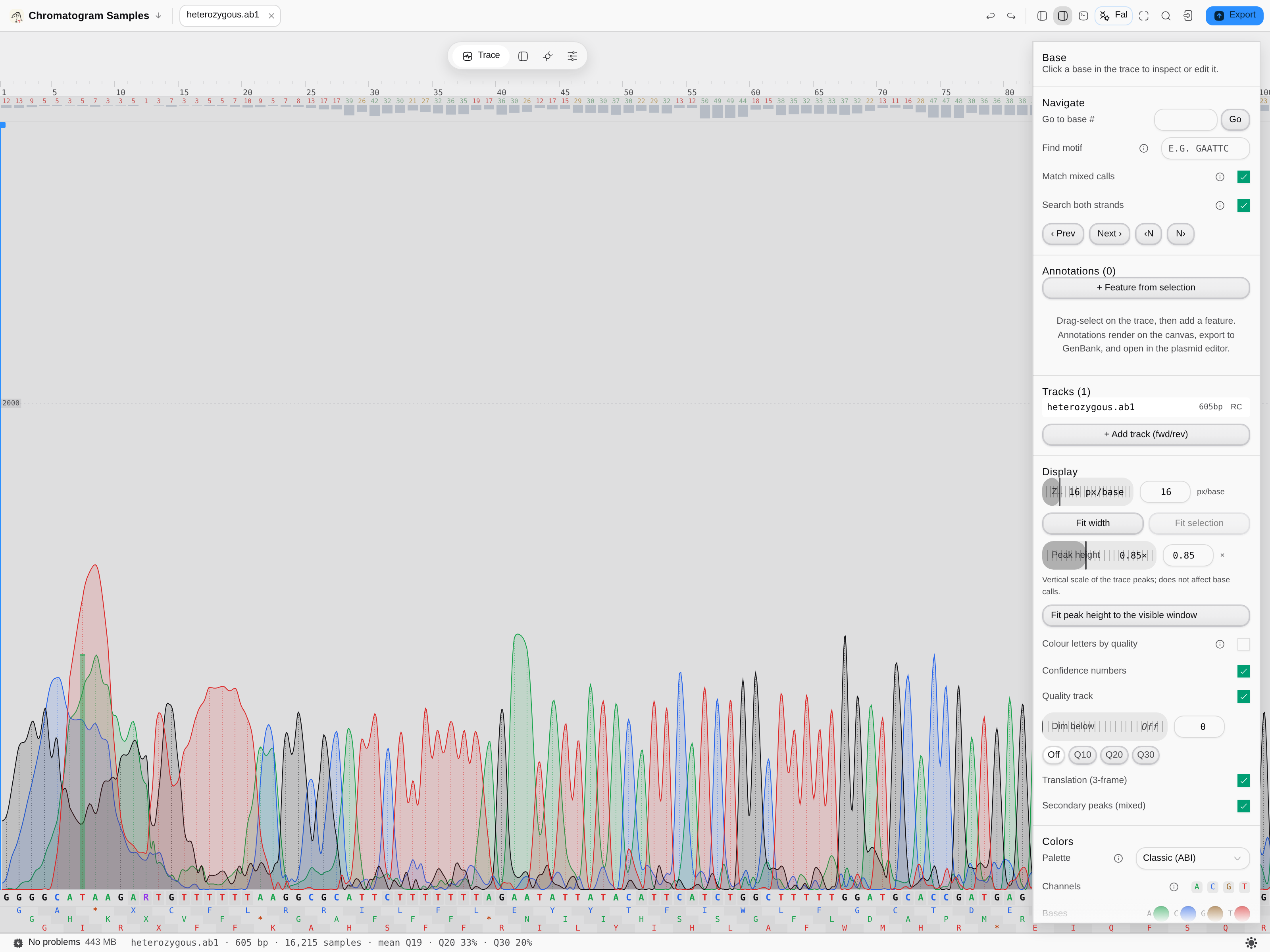
heterozygous.ab1 from the Trace samples starter — 605 bp · 16,215 samples · 33% of bases at Q20
and 20% at Q30, and the read's own quality is Q11.1, an expected 92.3% accuracy. The status bar
in this frame predates that reading and shows the arithmetic mean of the per-base scores, Q19, which
is the higher of the two numbers for the reason given above. The four dye channels are drawn as filled peaks with the called
base under each and the per-base confidence numbers above; the ambiguity codes in the base row
(R, Y, X) are where a second peak sits under the called one, with Secondary peaks (mixed)
on. The right rail carries every control that shapes the drawing — px/base, peak height, quality
track, dim-below threshold, 3-frame translation and the channel palette — none of them a hidden
default.
Related
Sequencing Verification grades a read against the sequence you designed. The reads in one tab can be aligned to each other in one action, and a clean consensus is what the sequence map then shows against your construct.