
Copy-number canvas
| Document kind | copynumber |
| Drawn from | a file — it can also be previewed in the file manager |
| Formats that open here | Affymetrix CNCHP · Affymetrix CYCHP · Affymetrix OSCHP · Affymetrix CHP |
| Refuses to draw below | 640px wide |
What it draws
Copy number along the genome, as the array measured it.
A microarray covers the genome with hundreds of thousands to millions of markers — short probes at known positions. Comparing each marker's signal against a reference gives a log2 ratio: zero where a region is present in the usual two copies, above zero where there are more, below where there are fewer. A whole chromosome of those ratios, plotted along its length, is what a cytogeneticist reads to find a deletion or a duplication.
Five regions, arranged the way a genome is actually navigated, each one a pane you can resize, maximise or drag somewhere else:
- a karyoview — every chromosome the file indexes, side by side, so a whole genome is one glance, with each chromosome's own calls marked beside it;
- the detail view for the selected chromosome, its graphs stacked over one shared base-pair axis, with the file's own segment calls in a lane beneath them;
- a segment table — every call the file made, one row each, with its cytoband, span and confidence;
- that chromosome's ideogram, the banded shape a karyotype is drawn as, for position context;
- a genome profile — all chromosomes at true relative length, with their calls painted along them, so a genome-wide pattern is visible without opening one chromosome at a time.
Everything on those five is one selection and one window: pick a chromosome anywhere and the rest follow it.
What opens in it
Affymetrix (Thermo Fisher) copy-number result files: CNCHP, CYCHP, OSCHP and the copy-number CHP. These are what the array's own analysis software writes — the calls have already been made, and this canvas reads them rather than recomputing them.
Raw intensity files (.CEL) do not open here. Turning raw intensities into copy number needs a
reference model built from hundreds of arrays; that is a different job from reading a result, and a
thin version of it would produce numbers that look like calls and are not.
Which graphs appear depends on the file, not on this page. A CNCHP carries log2 ratio, copy number state, smooth signal and allele difference. A CYCHP adds weighted log2 ratio, loss of heterozygosity and B-allele frequency. The list you see is the one your file actually contains.
What this computes
Every value below is read from the file, with one exception that is switched off until you ask for it: copy-number state calling, described at the end of this list.
-
Log2 ratio — the marker's signal against the reference, on a log2 scale.
0is the normal two copies;+0.58is three;−1is one. Scattered noise around zero is expected. -
Weighted log2 ratio — the same quantity after the analysis has down-weighted markers it trusts less, so a run of them reads more cleanly.
-
Smooth signal — a smoothed estimate of copy number itself, in copies rather than on a log scale. It is the line a reader follows to see where a segment starts and stops.
-
Copy number state — the integer number of copies the analysis called for that marker.
-
Allele difference — the difference between the two alleles' signals at a marker. In a normal diploid region heterozygous markers split into two bands and homozygous ones sit at the extremes; a region that loses one parental copy loses the split, which is how loss of heterozygosity shows itself.
-
Loss of heterozygosity — where the analysis called a stretch as having only one parental haplotype, whether or not the copy number changed.
-
Loss of heterozygosity, recomputed — the same question asked again from the array's own per-marker genotype calls, rather than read off the runs the producer wrote. A heterozygous call inside a truly homozygous stretch is a genotyping error, so the method asks how many heterozygotes a window of markers can hold before the stretch stops being explicable by error alone: the cutoff is a binomial tail against an assumed error rate, and the window width is then solved so that a true run of that width would be detected. Both the false-positive rate and the assumed error rate are yours to set, which is what makes this a second opinion rather than a second copy — the runs in the file came out of one tuning and cannot be re-asked. The window the values solved to is reported with the result, because two samples given the same setting get different windows: the width is solved against each sample's own heterozygosity. The error rate is re-estimated from the sample's own no-call rate where the genotype confidences warrant it, and the result says which value was used. Three ways a marker can go uncalled are reported separately and none of them is "no loss of heterozygosity here": a marker with no genotype call is dropped, a stretch shorter than the window is left unevaluated rather than called clear, and a chromosome the walk never reaches is reported as such. It needs an array that states genotype calls — an OncoScan result does; a CytoScan result carries the table with no rows in it, and the panel says so by name rather than reporting a genome with no loss of heterozygosity in it.
-
Somatic mutations — for an array that assays them, the producer's own call for each mutation probe set, the score it was called on, and the two thresholds that probe set was graded against, which differ row to row. The call is reported in the producer's own words rather than reduced to detected/not, so a confidence grade it states arrives intact. The file names each probe set but does not say where it is, so the gene, protein and cDNA change, COSMIC id and locus come from the array's own annotation database for the genome the file states. Each call is then drawn on the karyoview and in a Somatic calls lane of the detail view: a large dark circle where the mutation was detected, a small gray dot where the wild type was called. On GRCh37 the database writes each position one base before the variant (checked against the reference genome at Ensembl), so that position is corrected to the variant's own first base.
-
Allele-specific copy number (the allele split) — for a file whose analysis estimated it, how many copies of each parental allele a segment carries: a major and a minor count, so two copies read as 1+1 (both parents present) or 2+0 (one parent's copy duplicated, the other lost). That distinction is invisible to total copy number, and it is what the split is for. Each segment is named by what its split means: balanced (equal counts), allelic imbalance (unequal, both present), loss of heterozygosity (minor allele 0) and homozygous deletion (0+0). Loss of heterozygosity is placed against the sample's own ploidy as the analysis estimated it: at that ploidy it is copy-neutral (as in uniparental disomy), below it a loss, above it a gain. The split is only as good as the estimate of the aberrant-cell fraction behind it — the analysis assigns integer tumour copy numbers only where it could determine that fraction — so the fraction is shown with the result, and a file where it could not be determined states no split and says so. Segments the analysis did not estimate are listed as not estimated and are never read as 0+0. Over the estimated segments, the whole-genome summary a cancer genomics report quotes: fraction of the autosomal genome in loss of heterozygosity, the count, total size and largest homozygous deletion, the modal allele state, a whole-genome doubling call from it, a genomic instability score (the fraction of the autosomal genome away from the modal balanced state), and the size of segments with an odd copy number or a raw estimate halfway between integers. (Correctness provenance: every summary metric is checked against ASCAT's own implementation, segment for segment, on four public tumour arrays.) The canvas lists every segment with its split, raw estimates and state, and draws total and minor-allele copy number under the plots, so a copy-neutral loss of heterozygosity shows as a total on the two-copy line with the minor allele on the floor.
-
B-allele frequency — the proportion of signal from one of the two alleles. It is derived, not measured, and it is not the same quantity as allele difference; where a file supplies one it is drawn as the file supplies it and never relabelled as the other.
-
Copy-number segments (inferred, off by default) — where the copy number changes along a chromosome, and to what. A hidden Markov model runs over the log2 ratios: one state per copy-number level, each with a mean and a spread, and a single stickiness setting deciding how many markers of contrary evidence it takes to move a call. The most probable path through those states is found for the whole chromosome at once, so a single wild marker does not create a segment, and the result is drawn as a step line over the markers it was derived from — the step is the model's claim, the band beneath it is the evidence, and a claim the markers do not support is meant to be visible as a disagreement between the two.
Three things are stated with the result rather than assumed. The level means are a property of the array chemistry, not of biology — a single copy against two would be −1.0 on a log2 scale and the values in use are attenuated well short of that, so the panel names where they came from and you can see whether they apply to the file you opened. Markers with no value are not dropped: they are carried through the model, which lets their neighbours stand in for them, and the count is reported. A segment narrower than one pixel is drawn at its true width and is therefore invisible, so the count of those is reported too — otherwise the number of segments and the number you can see would disagree with no way to tell why.
It applies only to log2-ratio graphs. Running it on an allele difference or a raw signal would produce confident numbers about the wrong quantity, so those graphs do not offer it.
The calls themselves, as a table. Everything above is measured or inferred per marker; a report is written about regions. Every call the file made is listed as a row, and each row carries what a report names it by:
- Type — gain, loss, loss of heterozygosity, copy-neutral loss of heterozygosity, or mosaic. Copy-neutral loss of heterozygosity is its own type rather than a kind of LOH, because it means normal copy number with only one parental haplotype — the uniparental-disomy case, which a copy-number track alone cannot show.
- Location — the first and last marker of the run, in the file's own coordinates.
- Cytoband — the band the call starts in and the band it ends in, which is how a cytogenetic
report names a place:
p15.33 → p15.31. It needs a genome assembly, so with no assembly chosen the cell is empty rather than guessed. - Size — the bases spanned. A call on a single marker spans zero bases, and says so instead of being rounded up to a probe spacing that was never measured.
- Markers — how many markers carried the call. A large span over few markers is a weaker statement than the same span over many, and this is the column that says which you have.
- State — the copy number called for the region, where the file states one. A loss-of- heterozygosity call has none, because it is not a statement about copy number.
- Confidence — the analysis's own confidence in that segment, as the file records it. It is read, never computed here, and it is absent rather than assumed when the file does not carry it.
- Mosaic fraction — for a mosaic call, the estimated proportion of cells carrying the event, with its sign kept: the sign says whether the mosaic event is a gain or a loss, and dropping it would merge two opposite findings.
Selecting a row takes the rest of the canvas to that region, so a number in the table and the picture of it are one click apart.
Undefined values are drawn as gaps, not as zero. A marker with no allele difference is a marker the analysis could not call there — which is a result, and a different one from a difference of nothing.
Where the calls land — region overlap. A list of intervals is not yet a report. The last step is placing this sample's calls in the regions someone has decided matter, and there are two kinds of such list.
- Curated dosage regions. Recurrent regions of the genome, each scored for haploinsufficiency — does losing a copy cause disease — and triplosensitivity — does gaining one. A loss is read against the first score and a gain against the second; a stretch of homozygosity or a mosaic event is shown where it falls but no dosage score is claimed for it, because neither score is evidence about an event that changes no copy number. The scores are a vocabulary, not a scale: sufficient evidence, some evidence, little evidence, no evidence, autosomal recessive, dosage sensitivity unlikely — so nothing is sorted or thresholded on them. Regions the curators have not yet placed on your assembly are listed separately and are not reported as clean: they were not checked, which is a different answer from having nothing in them. (Correctness provenance: the regions, their scores and their citations are the ClinGen Dosage Sensitivity curation, cached with its curation and retrieval dates and shown with the ISCA identifier a report cites.)
- A region file of your own. The panel of loci your laboratory reports on, in the two formats a cytogenetics workstation writes one in — BED and AED. Every region in your file is listed, including the ones this sample has nothing in, because a region file is a checklist and nothing in 22q11.2 is the answer you came for. An AED carries your own typed columns beside the coordinates, and those are shown with each region rather than discarded. No dosage score is claimed for these regions, because nobody curated them: the overlap itself is the reading.
For each region you get the number of calls in it, the fraction of the region they cover between them — counted once per base, so two overlapping calls cannot sum past the whole — and, for the closest match, the reciprocal overlap: the smaller of the two containment fractions, so a focal call inside a whole-arm region scores low rather than scoring as a perfect match. No threshold is applied. Which overlaps are worth reporting is a laboratory's judgement, so every overlap is reported with the numbers to judge it by.
A region file must agree with the assembly in force, and is refused when it does not. A BED file carries no assembly of its own by specification, so the build is read from the track line a cytogenetics workstation writes there, and an AED states it as a metadata property. If the file names a different assembly than the sample, the regions are not read — the two assemblies place the same locus hundreds of kilobases apart, and a list silently placed on the wrong one still produces overlaps that still look like results. If the file names no assembly at all, that is said out loud and the build in force is used. Rows that cannot be read, intervals written end-first, and sequence names that had to be normalised are each counted and reported, because a region list that lost four rows quietly is worse than one that refuses.
Coding-sequence verdict — for the window in view, whether it contains a complete coding sequence (complete · partial · non-coding · none), read from the RefSeq gene models for the build, with how many of the widest transcript's coding bases the window holds. From a complete one, the spliced coding sequence (checked against NCBI's own coding sequences for both human builds) and its protein length. See A region's reference bases, and a gene's coding sequence below.
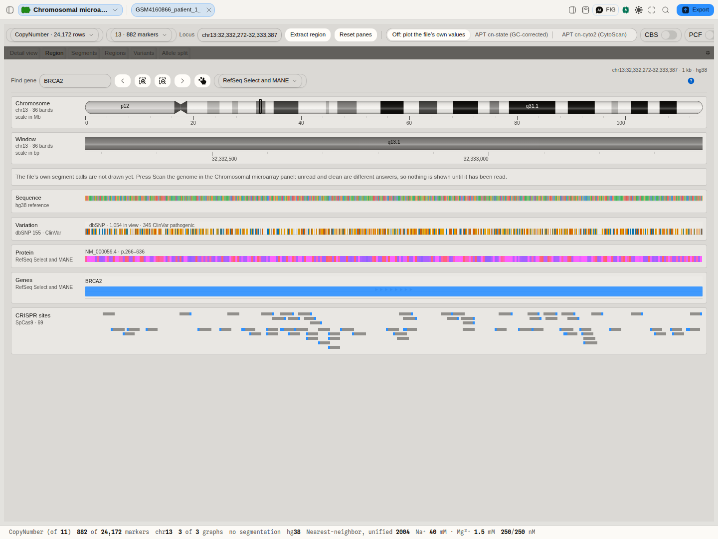
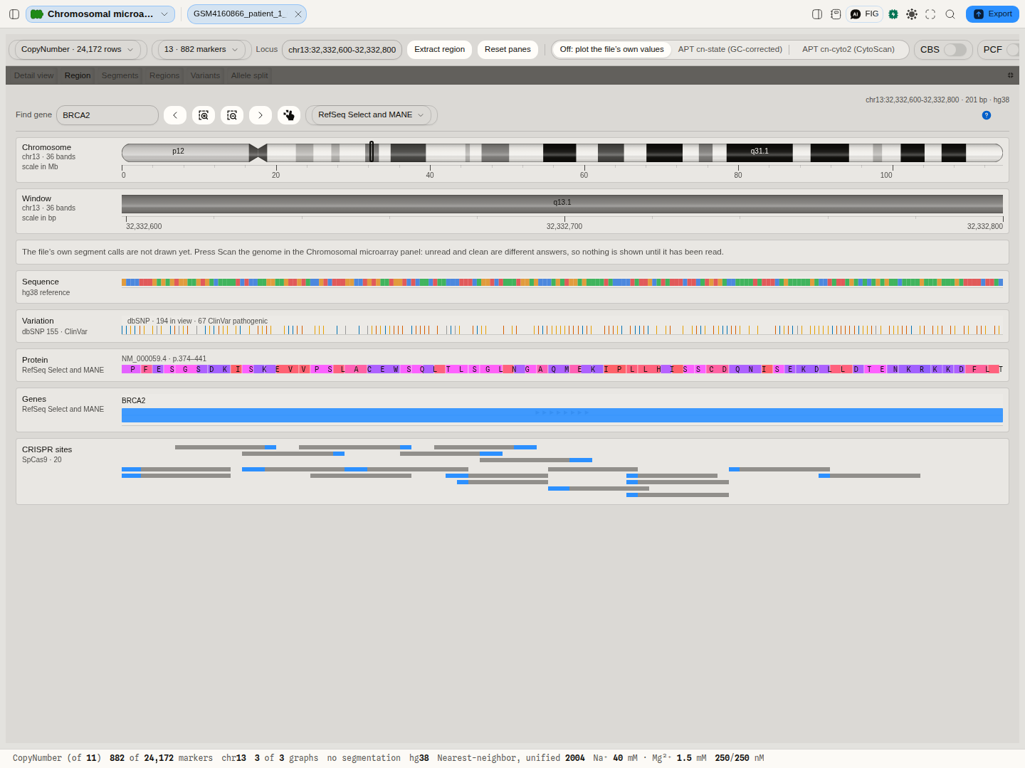
The region browser — for one window of the assembly, read live from the UCSC Genome Browser:
- Cytogenetic bands the window spans, and where it sits on the whole chromosome.
- Reference bases of the assembly, coloured by base.
- Known variants from dbSNP 155, with ClinVar's clinical significance (pathogenic, benign, other) as each mark's colour, and the counts in view.
- Encoded protein — for each RefSeq transcript, which residues the window encodes, numbered as
in the protein (
p.266–636), translated from the assembly's own bases with the chromosome's genetic code. A codon an intron splits is drawn in both of its pieces; the stop codon is marked and not counted as a residue. Checked residue by residue against NCBI's protein for BRCA2. - Transcripts from the RefSeq set chosen: RefSeq Select and MANE (one per gene), Curated, All, or Predicted.
- CRISPR sites on both strands for the chosen nuclease (SpCas9 by default, nine others offered): the spacer, the PAM, the cut position, and the Rule Set 1 and CRISPRscan on-target scores, which are SpCas9-trained and so are reported for SpCas9 only.
- Gene lookup — a gene symbol resolves to its MANE Select transcript (GRCh38), or to HGNC's location where an assembly has no MANE set, with a 2% margin either side.
Comparing two samples
One sample's copy number is read against a reference built from many arrays, so the plot already answers how does this genome differ from a normal one. The other question a laboratory has is how does it differ from that one — a tumour against its own normal, one patient against another, a case against a control run on the same platform.
Choose a second file under Compare with, and its markers are drawn behind this sample's on the same axis: the same chromosome, the same window, the same buckets. That sharing is the point. Two plots side by side answer what does each look like; one axis answers is this segment present in one and absent in the other at the same coordinate, which is the question the comparison exists for.
What the comparison states rather than assumes, because two files are two files:
- The chromosome is matched by name, not by number. These files state their own numbering — which number is X is written in the header and is not the same in every file — so the match is on the chromosome each file calls the same thing. A file that does not carry the chromosome you are looking at says so; it is a fact about that array, not an empty result.
- Graphs are matched by column name. A file that carries a different set of measurements is reported as carrying them, on the graph it cannot answer. Nothing is drawn from a column that happens to sit in the same position.
- Marker counts are stated separately for each sample. A different array covers a chromosome at a different density, and two envelopes over one axis must not let you assume one count for both.
- The vertical scale is fitted to both samples. Fitted to one, the other would be clipped wherever it goes further — and a clipped envelope does not look like a bigger excursion, it looks like agreement at the edge of the plot.
Nothing of the second file is read until you choose it, and then only the chromosome in view.
Regions a call is reported against
A call on its own is a span of DNA with a direction. What makes it a finding is where it lands: a 40 kb loss matters if it removes a gene that cannot be lost, and is unremarkable if it sits in a stretch that varies between healthy people. So the calls are laid over a region list — a set of named regions on a genome assembly — and every region is reported with what this sample has inside it.
Two lists are available, and the section states which one is in force.
The curated list, which is what you get without choosing anything. ClinGen's dosage-sensitivity curation: recurrent regions with ISCA identifiers, each scored for haploinsufficiency (the evidence that losing one copy causes disease) and triplosensitivity (the evidence that gaining one does), against published work the curation cites by PubMed identifier. A loss is read against the first score and a gain against the second. No score is claimed for a stretch of homozygosity or a mosaic call, because neither score is evidence about an event that changes no copy number — the overlap is still reported, what is withheld is the claim that a curated judgement grades it.
The score is a vocabulary, not a scale. ClinGen's values include 0, 1, 2, 3, 30 and 40, where 30 means gene associated with autosomal recessive phenotype and 40 means dosage sensitivity unlikely — so 40 is not "worse than 3", and nothing here sorts or thresholds on the number. The description is shown beside it, in the curation's own words.
Regions the authority has not placed on your assembly are named, not silently dropped. ClinGen publishes every region's location on GRCh37 and leaves a handful without GRCh38 coordinates. On GRCh38 those regions cannot be checked, and a list that quietly reported the rest would tell you your sample is clean in regions nobody looked at.
Your own region list. A laboratory reports against the panel it validated, and that panel is a BED file: named intervals on an assembly, which is the same file a genome browser takes as a custom track. Choose one under Region list and the sample's calls are placed in your regions instead. A BED line carries no dosage score, and the section says so once rather than printing "no score applies" under every row: your list says where to look, and claims nothing about what a change there means.
The assembly is the one thing a BED can get silently wrong, so it is the one thing that is
refused. BED's three required fields are the sequence name, the start and the end — none of them is
the genome build — and a file may state one only on an optional track line. If it states an
assembly that is not the one your sample is being read on, nothing is placed: the same band sits
hundreds of kilobases apart on two assemblies, and nothing on the screen would show the difference.
If it states none, its regions are placed on the build in force and the section tells you that is
what happened. Lines that are not BED records are counted and quoted with the reason, so a panel of
forty regions arriving as thirty-eight cannot pass unnoticed, and a list whose sequence names never
meet your sample's is reported as unchecked rather than as clean.
What is computed for each region
- Calls inside it — how many of this sample's calls fall in the region at all, by type.
- Reciprocal overlap — the shared bases as a fraction of the LARGER of the two spans, so a small focal call inside a whole-arm region scores low rather than reporting as a full match. It is the measure that says whether two intervals describe the same event.
- Region covered — the fraction of the region the calls cover between them, counting each base once, so overlapping calls cannot add up past the whole.
- The dosage judgement, where the list carries one and the call's direction is one it speaks to.
No cut-off is applied to any of it. The obvious convention calls a region "hit" at 50 % reciprocal overlap; that number is a reporting convention, it differs between laboratories and indications, and choosing one here would put a threshold in your result that you did not set. Every overlap is reported with its numbers.
Correctness provenance: the curated regions are ClinGen's own published curation, cached with its curation date and retrieval date; the interval arithmetic is checked against bedtools, the reference implementation of BED interval operations.
The region browser
The Region tab is a genome browser under the copy-number result, modelled on the browsers genome engineers use to plan an edit: the chromosome with the window marked, a ruler, and one lane per kind of evidence beneath it, all on one base-pair axis. It follows the detail view's window, so selecting a call, typing a locus or dragging on the plot moves it too. Find gene takes a symbol and goes there, onto another chromosome if it has to. The arrows pan by half a window, the magnifiers zoom by two, and the last button returns to the whole chromosome.
Each lane reads only up to the width at which it can still be read, and says so above it rather than drawing nothing: transcripts and known variants up to 1 Mb, bases and protein up to 100 kb, CRISPR sites up to 10 kb. A window holding more than 2,000 known variants is refused rather than drawn as one solid band. The protein lane draws residue letters from 360 bp down, and the bases lane draws a base once one is at least a pixel wide.
The window needs a genome build. A file that states none uses the one chosen for the cytoband overlay; with none chosen, the tab says so instead of guessing.
Uncertainty and quality
The file carries the array's own quality measurements, and they are shown as the file states them with no pass or fail attached: MAPD (how much neighbouring markers disagree — the standard noise measure for these arrays), SNP QC, and the call rate. Published acceptance thresholds exist, but they are stated by the manufacturer for particular array types, so applying them to a file that may be a different type would be an assertion this page has no basis for.
Controls
- Data set — which table in the file to plot, where it holds more than one.
- Chromosome — which one the detail view and the ideogram show. Selecting a cell in the karyoview does the same thing.
- Graphs — one switch per graph the file carries.
- Cytobands — which genome assembly's banding pattern to draw.
- Region list — which set of regions the calls are reported against: the curated list, or a BED file in your project.
- Compare with — a second copy-number file in your project, drawn behind this one on the same axis and the same buckets.
- Segment table — sort by any column, or filter by typing part of a location, a cytoband or a call type. Sorting by location is genomic order, not alphabetical order, so chromosome 9 comes before chromosome 10.
- Recompute loss of heterozygosity — runs the method again on the file's own genotype calls, with three settings: the false-positive rate the heterozygote cutoff is set against, the assumed genotyping error rate, and the shortest run worth reporting in base pairs. Offered only where the file states genotype calls.
- Panes — drag any divider to resize, maximise a pane to fill the canvas, or pull a tab out to see two things at once. The arrangement is remembered, and there is one action to put it back.
No assembly is chosen for you, and that is deliberate. These files identify the annotation release they were analysed against, not the genome assembly itself, and the two are not the same statement. Drawing markers from one assembly against another's bands would move every one of them, and nothing on the screen would look wrong. So the plot is drawn from the file's own coordinates — always correct, whatever the file was built against — and the banding pattern is an overlay you switch on by naming the assembly, with the file's own annotation string shown beside the control so the choice is an informed one.
Taking the calls somewhere else
Three files come out of the canvas, and all three are the calls the file itself made rather than anything inferred here.
- Segment calls, as a table. One row per call, with its chromosome as the file names it, the start and stop positions exactly as the file states them, the marker count, the copy-number state and its label, the producer's own confidence, and the mosaic fraction with its sign. A field the file does not state is left empty rather than filled with a zero — a zero in the state column would read as a homozygous deletion on every stretch of homozygosity.
- Segment calls, as a genome-browser track. The same calls in BED, ready to open in IGV or
the UCSC Genome Browser or to intersect with
bedtools. BED counts from zero and excludes its end position while an array states the first and last marker of a run inclusive, so the coordinates are converted once, by the same conversion used everywhere a call is intersected with a curated region — the numbers in this file and the overlap figures on screen cannot disagree. Each call is coloured by what it is, in the same colour-vision-safe palette the canvas paints, and carries the producer's confidence in the score column. The assembly travels with it when the file names one: a BED's required columns cannot carry a genome, so it is written on the track line, which is where a browser looks for it. If the file names no assembly, none is written — the calls are still correct in the file's own coordinates, and nothing is asserted about which genome they sit on. - A chromosome summary. One row per chromosome that was actually read, with its markers and the counts and spans of each kind of call.
Nothing is written before the genome has been scanned, and the refusal says which it is: a genome that was read and carries nothing is a result, and a genome nobody has read is not.
A BED that names an assembly on its track line keeps it on the way back in, too — bring one into a project and the assembly it names is shown with it. A file that names none says so rather than being silently placed on whichever genome happens to be loaded.
Where it appears
As a document: open one of these files from a project and it draws on the stage. It also previews in the file manager, where the controls and the file's own facts appear beside the plot.
Performance and limits
These files are large — a CytoScan array is tens to well over a hundred megabytes, and carries millions of markers.
Opening one does not read it. The file carries its own per-chromosome index, so the header and that index are all that is read to draw the karyoview; a chromosome's markers are read only when that chromosome is selected. A whole genome's worth of measurements is never pulled into memory to show you an overview of it.
The plot is reduced to what a screen can show, one bucket per pixel column, keeping each bucket's highest and lowest value as well as its average. Keeping the extremes is the point: a single marker standing far above its neighbours is a focal amplification, and an average alone would flatten it into the baseline it stands out from.
The vertical scale fits the data rather than sitting at a fixed range, because the useful range differs between a log2 ratio and a copy-number state, and between one array type and another.
A region's reference bases, and a gene's coding sequence
With a genome build in force, the window the detail view is on can leave the canvas as a sequence. Extract region fetches that window's bases from the UCSC Genome Browser for the build and opens them as an editable record. They are the assembly's bases, not this sample's: an array measures dosage, not sequence, so a variant in this sample is not in them, and the record says so.
The selection box also reads the window against the RefSeq gene models for the build, where each transcript's exons and coding start and stop are declared by NCBI rather than inferred here, and gives one of four answers:
- Complete. The window contains at least one transcript's whole coding sequence. Pick the transcript (grouped by gene, longest protein first; this ordering does not mean the first is the canonical transcript) and Open CDS splices its coding exons out of the reference, reverse- complementing a minus-strand gene, and opens the result as its own record with one CDS feature over every base. Tools that work residue by residue, such as site-directed mutagenesis, read it directly. The spliced bases are checked before anything opens: they must end in a stop codon and contain none before it, or the action refuses and names the codon, because a RefSeq transcript can differ from the genome it is placed on.
- Partial. The window holds some coding bases but no complete coding sequence. A focal loss inside a gene is the usual case. A fragment has no reading frame of its own, so nothing is offered, and the box says how many of the gene's coding bases the window holds.
- Non-coding. The window overlaps genes but no coding base: an intron, an untranslated end, or a non-coding RNA.
- None. The window overlaps no annotated transcript.
A transcript whose coding sequence is not a whole number of codons (RefSeq marks a few hundred of these as incomplete at one end) is never offered, even when the window contains all of it.
Screenshots
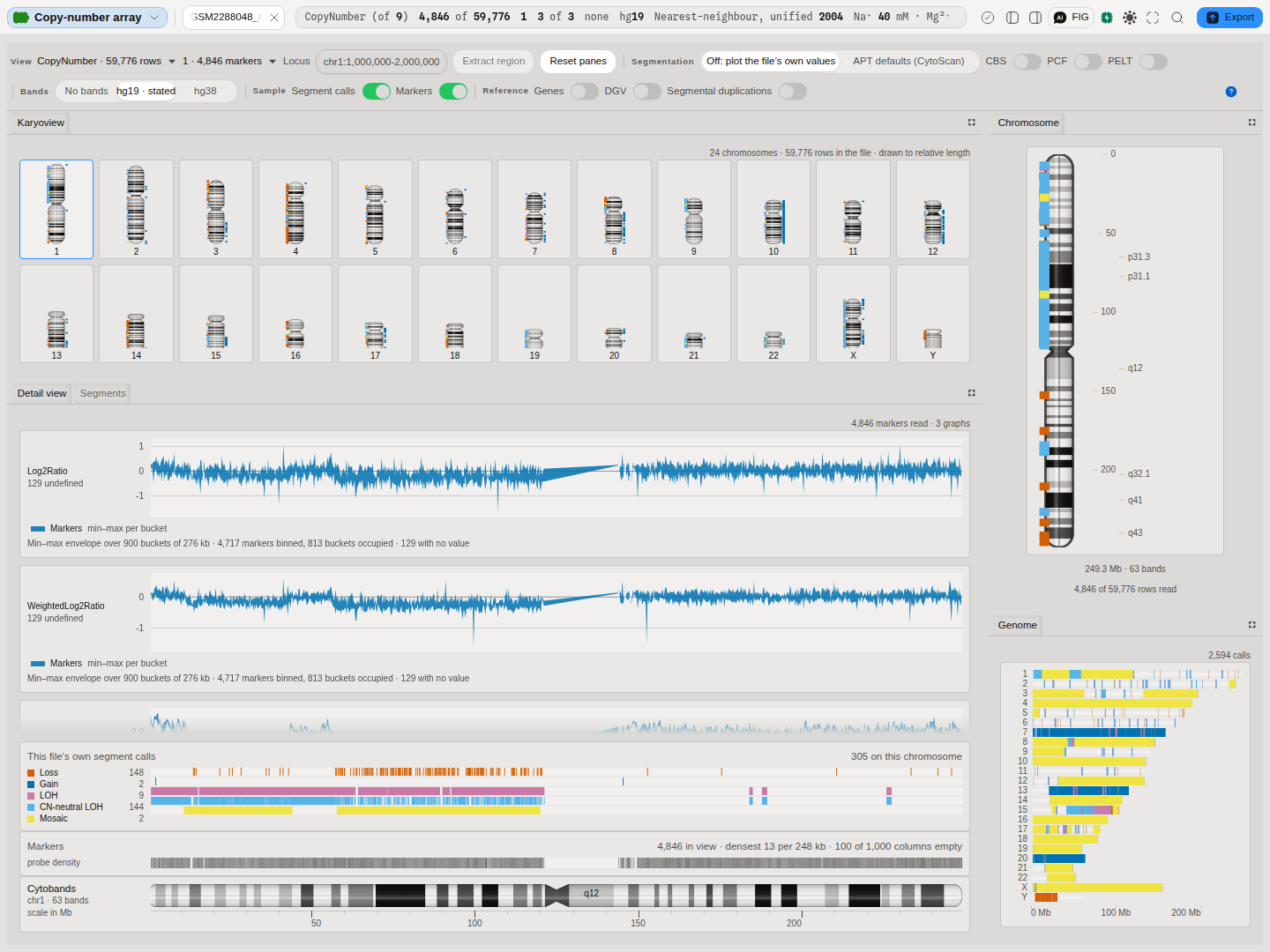
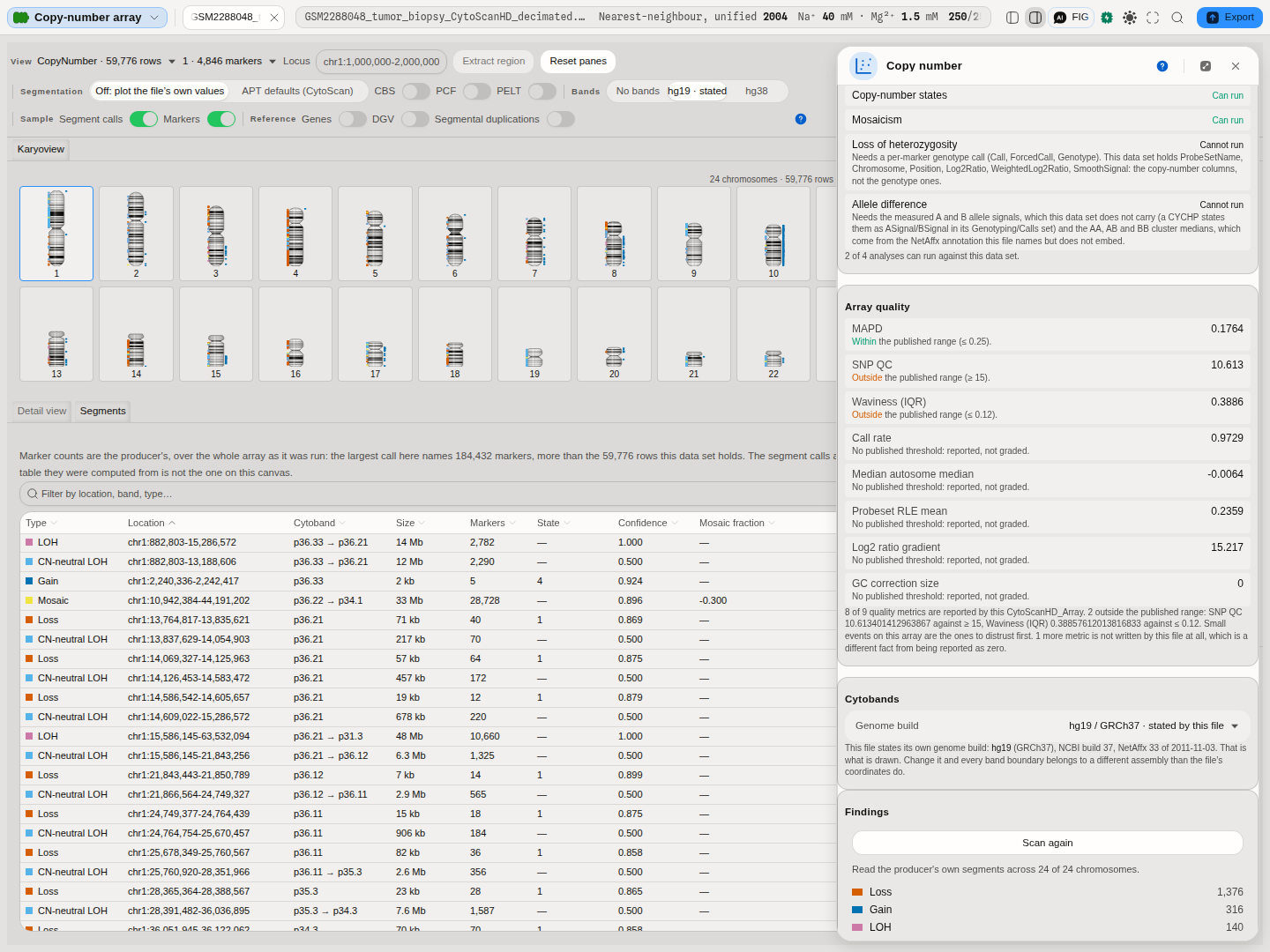
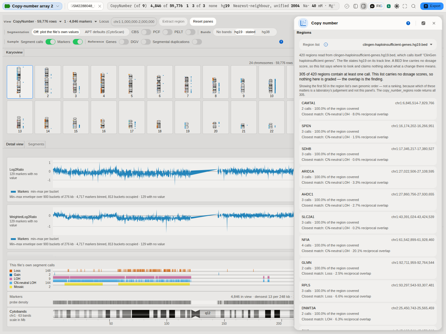
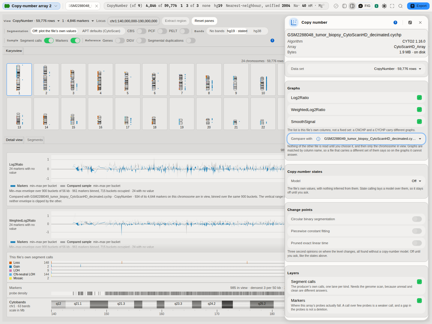
The first two frames above are the same file at the two resolutions this canvas exists to hold together: the picture, where a pattern across a genome is one glance, and the list, where a single call carries the numbers a report is written from. Selecting either takes the other to it.
Related
- Karyoview and ideograms — this page.